Homework: Intro to R

Author

Jelmer Poelstra

Published

March 4, 2024

1 Why R?

R is a versatile, open source programming/scripting language that’s particularly useful for statistics and data visualization.

Yes, there is a learning curve, and many of us just want to get on with our analysis –
but investing in learning R will pay off:

R gives you greater flexibility to do anything you want.
A greater reproducibility of scripting vs clicking.
R is highly interdisciplinary – e.g. very useful for analyzing sequencing data but can also be used to create maps and perform GIS analyses, and so on!
R is more than a platform to perform analysis. Combined with Markdown (a simple text markup language), you can use R to produce sophisticated reports, and create slide decks and websites such as this one!

Furthermore, R:

Is freely available on all platforms, and open source.
Has a large and welcoming user community.

Learning Objectives

Get some basic familiarity with R and RStudio
Learn why and how to use RStudio Projects
Understand objects, functions, and how to use them
Understand the concepts of vector and data.frame
Explore the structure and the content of a data.frame
Learn to subset/slice vectors and data frames
Learn about how R handles missing data

2 Getting set up

2.1 Start an RStudio session at OSC

Log in to OSC at https://ondemand.osc.edu.
Click on Interactive Apps (top bar) and then RStudio Server (all the way at the bottom).
Fill out the form as follows:
- Cluster: Pitzer
- R version: 4.3.0
- Project: PAS2714
- Number of hours: 4
- Node type: any
- Number of cores: 1

Click to see a screenshot

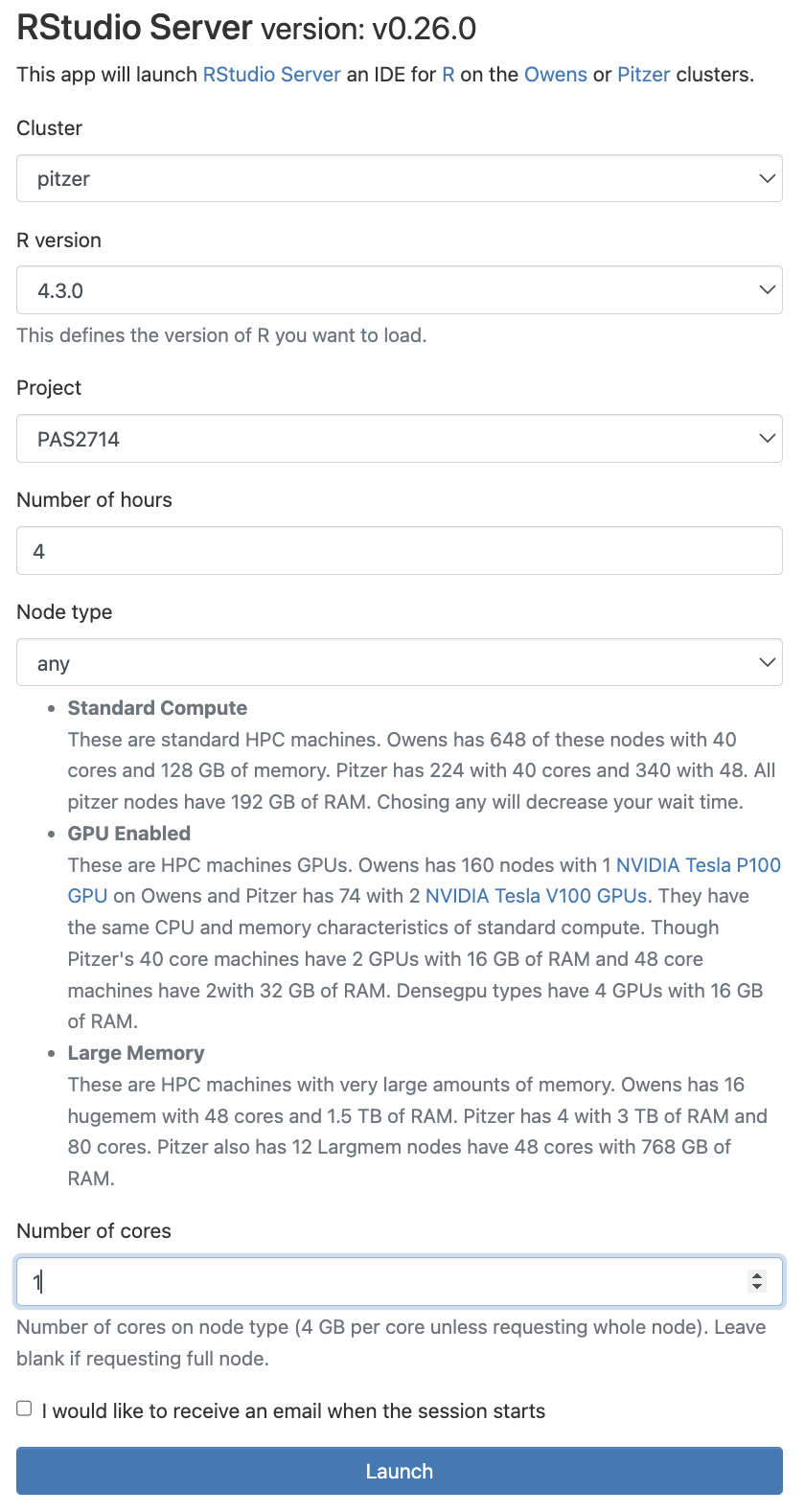
Click the big blue Launch button at the bottom
Now, you should be sent to a new page with a box at the top for your RStudio Server “job”, which should initially be “Queued” (waiting to start).

Click to see a screenshot

Your job should start running very soon, with the top bar of the box turning green and saying “Running”.

Click to see a screenshot

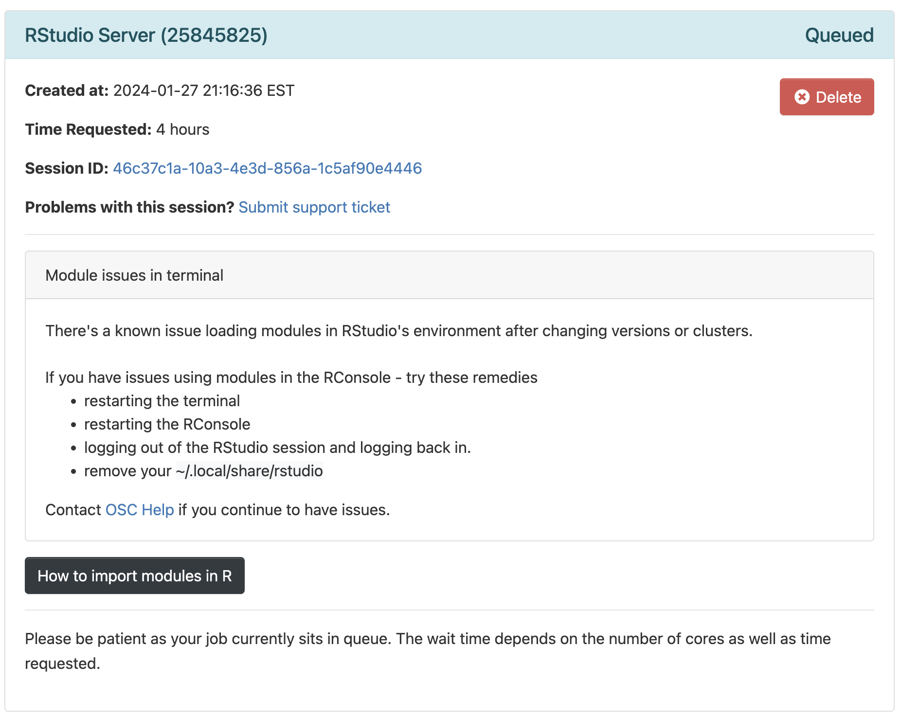
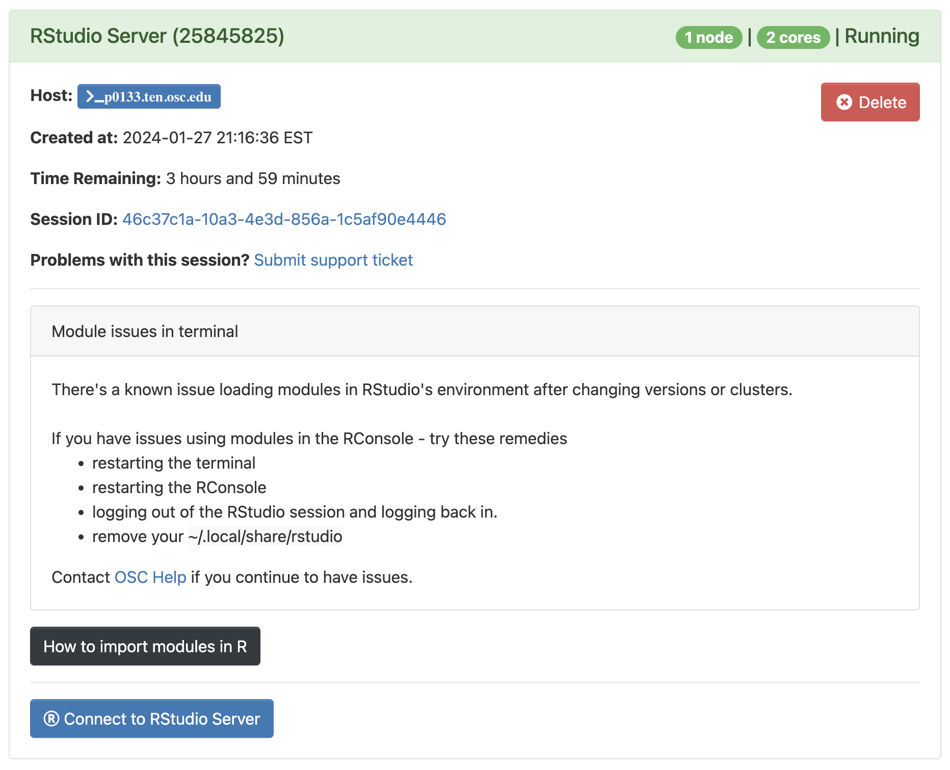
Click Connect to RStudio Server at the bottom of the box, and an RStudio Server instance will open in a new browser tab. You’re ready to go!

2.2 R vs. RStudio

R simply provides a “console” to type your commands. However, because we want to save our commands in scripts, examine output such a graphics, and so on, we would like an environment that provides all of this side-by-side.

We will use RStudio, an excellent “Integrated Development Environment” (IDE) for R. In RStudio, we have a single interface to write code, navigate files on our computer, inspect the objects we create, and visualize plots.

RStudio is divided into 4 “panes”¹:

Top-left: The editor for your scripts and documents.
Bottom-left: The R console.
Top-right: Your environment/history.
Bottom-left: Your files/plots/packages/help/viewer.

3 Interacting with R

3.1 R as a calculator

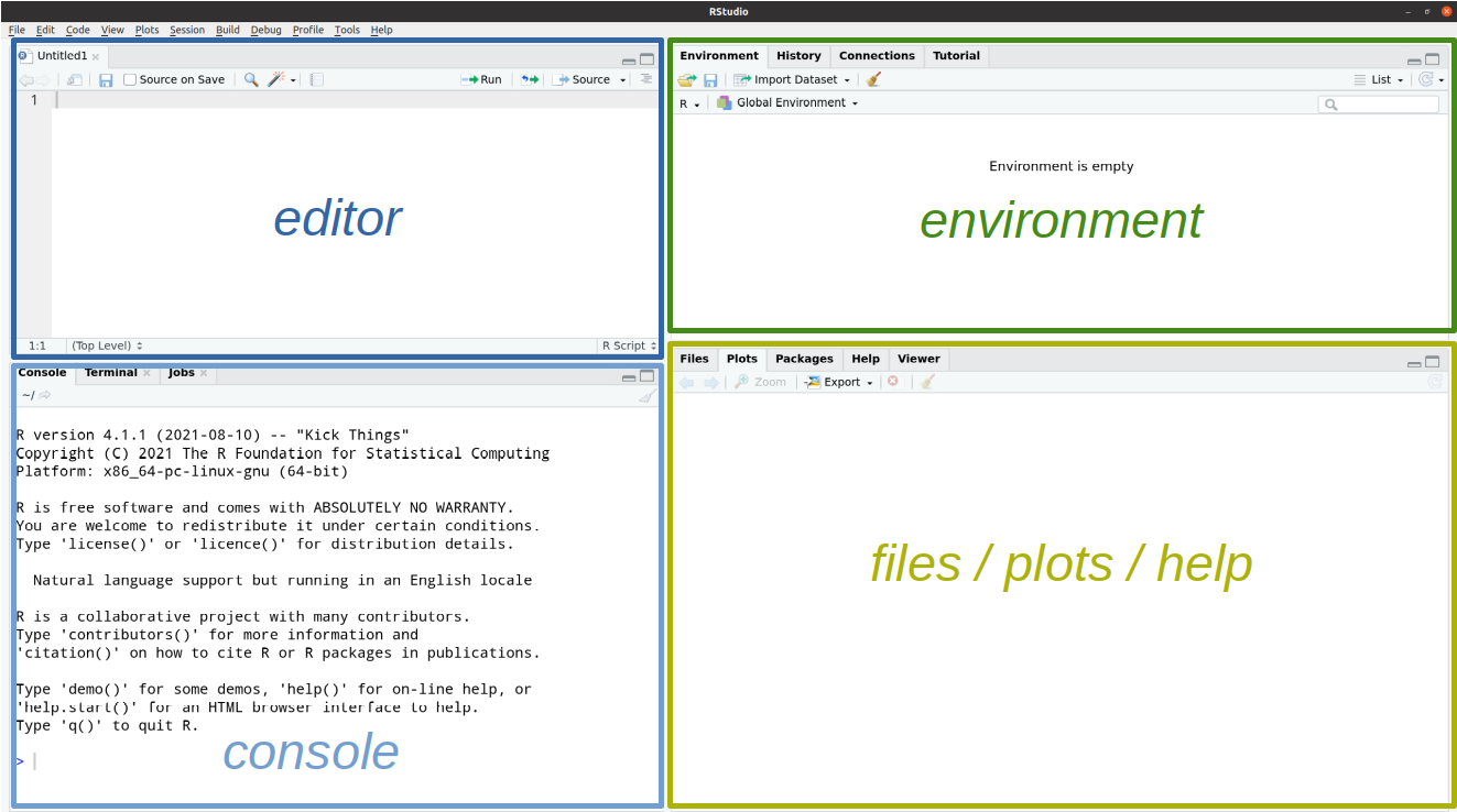
The lower-left RStudio pane, i.e. the R console, is where you can interact with R directly. The > sign is the R “prompt”. It indicates that R is ready for you to type something.

Let’s start by performing a division:

203 / 2.54

[1] 79.92126

R does the calculation and prints the result, and then you get the > prompt again. (The [1] may look a bit weird when there is only one output element; this is how you can keep count of output elements.)

With the standard symbols you can use R as a general calculator:

203 * 2.54   # Multiplication

[1] 515.62

203 + 2.54   # Addition

[1] 205.54

3.2 Trying some random things…

   203     - 2.54

[1] 200.46

This works: so R just ignores any extra spaces. How about:

203 +

Now the prompt is a +. What is going on? (Click for the answer)

R is waiting for you to finish the command, since you typed an incomplete command: something has to come after the + to be added to what came before.

While it was obvious here, you will often type incomplete commands without realizing you did so. Just remember that when you see the + prompt, you are missing something in your command: often, you’ll have forgotten a closing parenthesis ) or you accidentally opened up an unwanted opening parenthesis (.

Press the Esc button to get your prompt back.

And if we just type a number:

[1] 203

R will print the number back to us! It turns out that the default, implicit action that R will perform on anything you type is to print it back to us (it is calling a function called print() under the hood).

Rather than a number, what if we want R to print back to us some text, which in programming lingo is called a “character string”?

Fantastic

Error in eval(expr, envir, enclos): object 'Fantastic' not found

What seems to be going wrong here? (Click for the answer)

Whenever you type a character string, R expects to find an “object” with that name. (Or, if you would use parentheses after the string, like string(), it will expect a function.)

Because no object called Fantastic exists, R throws an error. To refer to a literal string instead, we need to use quotes (see below).

We can get R to print character strings back to us, and work with them in other ways, as long as we quote the strings:

"Fantastic"

[1] "Fantastic"

"I'm really liking R so far."

[1] "I'm really liking R so far."

So, R treats numbers and character strings differently: unlike numbers, character strings need to be quoted. This avoids confusion with objects (we’ll learn about those in a minute) because unquoted character strings are assumed to be objects, and also allows for “special characters” like spaces.

Quote types

Double quotes ("Fantastic") and single quotes ('Fantastic') can be used interchangeably in R. Double quotes are preferred by most “style guides”.

4 Getting Organized

4.1 Need for Scripts and RStudio Projects

We can go along like this, typing commands directly into the R console. But to better keep track of what you’re doing, it’s a good idea to write your code in files, i.e. “scripts”. And when we start creating scripts, we need to worry about how we organize the scripts and data for a project.

It is good practice to keep a set of related data, analyses, and text self-contained in a single folder, and use that folder as the working directory — in the Unix shell and in R alike. RStudio provides a helpful way to keep your working directory constant through its “Projects”. When you use a Project, your working directory will be the top-level directory of that project.

4.2 Create a new RStudio Project

To create a new RStudio Project inside your personal dir in /fs/ess/PAS2714/users (e.g., for me, the dir /fs/ess/PAS2714/users/jelmer)

Don’t have a personal dir there? (Click to expand)

If you followed the shell homework, you should have created your own dir within /fs/ess/PAS2714/users.

If you don’t have one, you can quickly create it as follows:

dir.create(paste0("/fs/ess/PAS2714/users/", Sys.getenv("USER")))

Click File (top bar, below your browser’s address bar) > New Project
In the popup window, click Existing Directory.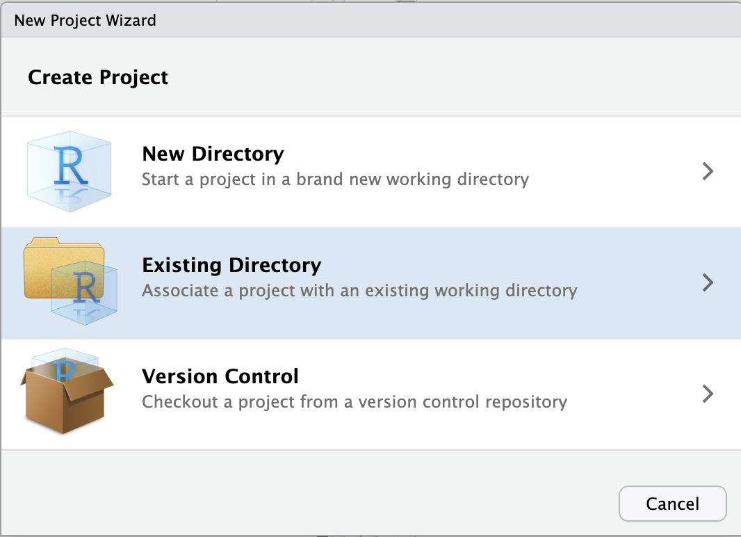

Click to see a screenshot

Click Browse... to select your personal dir.

Click to see a screenshot

In the next window, you should be in your Home directory (abbreviated as ~), from which you can’t click your way to /fs/ess! Instead, you’ll first have to click on the (very small!) ... highlighted in the screenshot below:

Type at least part of the path to your personal dir in /fs/ess/PAS2714/users, e.g. like shown below, and click OK: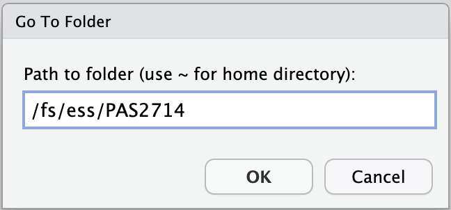

Now you should be able to browse/click the rest of the way to your personal directory, something like /fs/ess/PAS2714/users/jelmer.
Click Choose to pick your selected directory.
Click Create Project.

RStudio should reload and you should now have your new Project “open”. Your working directory should be the Project’s directory. We can check this using getwd():

getwd()

/fs/ess/PAS2714/users/jelmer

From now on, we will not change our working directory, and refer to all files relative to our project’s top-level directory.

4.3 Create an R script

Create a new R script (File > New File > R Script)
Click File > Save As to save the script in the scripts dir that you should see within your personal dir.² Give it a descriptive name like intro-to-R.R.

From now on, type your commands into this script and execute the commands from there.

To send code from your script to the console, press Ctrl/Cmd + Enter. This will copy the line of code that your cursor is at to the R console and execute it, and then the cursor will move to the next line.

4.4 Commenting

You can use # signs to comment your code:

# Divide by 2.54 to get the wingspan in inches:
203 / 2.54    # Original measurement was in cm

Anything to the right of a # is ignored by R, meaning it won’t be executed
You can use # both at the start of a line (entire line is a comment) or anywhere in a line following code (rest of the line is a comment)
In your R script, comments are formatted differently so you can clearly distinguish them from code

We recommend that you use lots of comments in your R scripts! They are useful not only for others that you may share your code with, but also for yourself when you look back at your code a day, a month, or a year later.

5 R objects

5.1 Assigning stuff to objects

We can assign pretty much anything to an object with the assignment operator, <-³. (This is a smaller-than sign < followed by a dash -.)

A few examples:

wingspan_cm <- 203
conversion <- 2.54

Type that into your script, and use Ctrl/Cmd + Enter twice to send it to the console.

The Environment tab

The objects you create get added to your “environment”, which RStudio shows in the Environment tab in the top-right panel — check that wingspan_cm and conversion are indeed there.

After you’ve assigned a number to an object, you can use it in calculations like so:

wingspan_cm / conversion

[1] 79.92126

Or, similarly:

wingspan_inch <- wingspan_cm / conversion
wingspan_inch

[1] 79.92126

This illustrates that when you execute code with objects, R substitutes the object name that you provide by its contents under the hood. In other words, the object is just a reference to the underlying value(s).

5.2 Object names

Objects can be given almost any name such as x, current_temperature, or subject_id. Some pointers on naming:

Because R is case sensitive, wingspan_inch is different from Wingspan_inch!
An object name cannot contain spaces — so for readability, you should separate words using:
- Underscores: wingspan_inch (this is called “snake case”)
- Periods: wingspan.inch
- Capitalization: wingspanInch or WingspanInch (“camel case”)
You will make things easier for yourself by naming objects in a consistent way, e.g. by sticking to a case type.
Object names can contain but cannot start with a number: x2 is valid but 2x is not⁴.
Make object names descriptive yet not too long — this is not always easy!

Exercises: objects and strings

A) Which of the following do you think would work and which would return an error:

session_topic <- "introduction"

session_topic <- introduction

Try both to see which works and what error you get for the other one. Also, try to describe in words what the correct line of code is doing.

Solution (click here)

The first of the two options was correct R code, while the second returns an error.

In general, keep in mind that unquoted character strings represent objects whereas quoted character strings are “literals”. Here, we wanted to assign the literal string "introduction" to the object session_topic — so the former should be quoted and the latter not.

An error is produced when you run the second option, because the object introduction does not exist (unless, of course, you had created an object of that name!):

session_topic <- introduction

Error in eval(expr, envir, enclos): object 'introduction' not found

B) Having run the code above, which of the following would make R print "introduction"?

"session_topic"

session_topic

Solution (click here)

The second option is the correct one: here, we want to have R print the value of the object session_topic (which we had just created in exercise A), so we shouldn’t use quotes.

session_topic

[1] "introduction"

C) Do you think the following code would successfully add 5 and 7? If not, what might happen instead?

"5" + "7"

Solution (click here)

In the code above, the “numbers” are saved not as numbers (in R lingo: as a numeric) but as character strings (character).

R can’t add character strings, so it will return an error:

"5" + "7"

Error in "5" + "7": non-numeric argument to binary operator

(Perhaps you expected it to combine/“concatenate” the two strings in some way — this is in fact what Python would do. Or to automatically convert the characters to numbers, since you’re clearly wanting them to be numbers — but it doesn’t do that either.)

D) (Bonus) What is the value of y after running the following lines of code?

x <- 50
y <- x * 2
x <- 80

Solution (click here)

Objects don’t get linked to each other, so if you change one, it won’t affect the values of any others. Therefore, y will keep the value 100.

6 Functions

Earlier, we divided 203 by 2.54, but what if we wanted to round the resulting number? Like for many things you may want to do in R, there is a function for that.

Functions are used by typing their name followed by parentheses:

round(203 / 2.54)

[1] 80

Here, round() is a function that rounds a number. The value in the parentheses is called a function “argument”, which is used in the execution of the function.

6.1 Using named arguments

Functions can have more than one argument, and some of them may have default values.

There are some functions that take many arguments and it can get confusing trying to keep them in order. In that case, it is better to explicitly name the arguments.

When you type a function name and pause for a moment, the arguments, their names, and their default values (i.e., the value if the argument is left unspecified) will be shown.

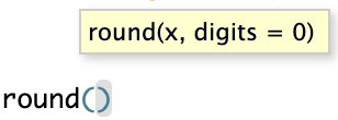
What is the second argument for round() and what is its default value? (Click here)

round has a second argument digits whose default is 0, such that numbers will be rounded to whole integers.

Below is an example using named arguments with round(). When the arguments are named, the order doesn’t matter! You might also enter the first few important arguments positionally, and later ones by naming them.

round(x = 1.538462, digits = 2)

[1] 1.54

round(digits = 2, x = 1.538462)

[1] 1.54

round(1.538462, digits = 2)

[1] 1.54

Also here, we can directly plug in objects:

wingspan_in <- 203 / 2.54
round(wingspan_in)

Or “nest” functions — here we are adding the log() function to compute the natural log:

log(round(203 / 2.54 ))

What is the order of execution in the last command? (Click for the solution)

round() is executed first, and the output of round() is used as the input of log().

7 Getting help

As we saw, when we typed round and paused for a moment, we got a pop-up with information about the function. Alternatively, you could type:

?round

… and the documentation for the function will show up in the lower-right pane.

This documentation is often a bit too detailed, and can be terse, so it takes some practice to read. Usage, Arguments, and at the bottom, Examples, are most useful.

Googling, even if you don’t know whether a function exists, will work too (e.g. “rounding a number in r”).

8 Vectors

A vector is the most common and basic data structure in R, and is composed of a series of values of the same type⁵. We can assign a series of values to a vector using the c() function (for “combine”). For example:

wingspans_cm <- c(11.8, 203, 18.2, 27.9)

A vector can also contain characters – but again, quoting is important, or R will think the strings are objects:

birds <- c("hummingbird", "bald_eagle", "chickadee", "cardinal")

As mentioned, all of a vector’s elements have to be of the same type of data. The function class() indicates what kind of data you are working with:

class(wingspans_cm)

[1] "numeric"

class(birds)

[1] "character"

8.1 Data types in R

The classes we saw above are different types of atomic vectors, R’s simplest data type. The 4 most common atomic vector types are:

"numeric" (or "double") – floating point numbers (numbers with decimals)
"integer" – integer numbers (no decimals)
"character" – character strings
"logical" – TRUE and FALSE (also known as boolean)

Also worth mentioning in this context is:

factor – Character strings with a discrete set of possible values, used mostly for statistical tests and plotting⁶.

Side note: Vector coercion – when not all elements are of the same type. (Click to expand)

What happens if we try to mix vector types (e.g., “character and numeric”) in a single vector? R converts them to all be the same type, and it does so without telling us about it. For example:

num_char <- c(1, 2, 3, "a")
class(num_char)

[1] "character"

8.2 Vectorization!

Let’s say we wanted to convert our vector of wingspans to inches: dividing each length in centimeters by 2.54. It turns out that this is as easy as dividing the vector by 2.54:

# wingspans_cm <- c(11.8, 203, 18.2, 27.9)  # Still working with the same wingspans_cm vector

wingspans_in <- wingspans_cm / 2.54
wingspans_in

[1]  4.645669 79.921260  7.165354 10.984252

This works because R “vectorizes” operations whenever it can. This means that in this case, each element in the vector weights_cm will be divided by 2.54 – this number is recycled to match the number of weights. Very useful!

Similarly, we can use two vectors of equal length to quickly operate on each element of the vector:

sizes_cm <- c(7.62, 90, 13.1, 21.8)

ratio <- wingspans_cm / sizes_cm
ratio

[1] 1.548556 2.255556 1.389313 1.279817

Exercise: Temperature conversion

Recall that you can convert a temperature of, for example, 26 Fahrenheit to Celcius as follows:

# (26°F - 32) / 1.8 = -3.3°C
(26 - 32) / 1.8

[1] -3.333333

Create and store a vector with the values 26, 21, 24, 32, 33, 41, 51, representing temperatures in Fahrenheit.

Now convert all the values in this vector from Fahrenheit to Celcius.

Click here for the solution

Thanks to R’s vectorization, you don’t have to convert these values 1-by-1:

temps_f <- c(26, 21, 24, 32, 33, 41, 51)

(temps_f - 32) / 1.8

[1] -3.3333333 -6.1111111 -4.4444444  0.0000000  0.5555556  5.0000000 10.5555556

8.3 Other data structures in R

While vectors can be composed of one of several data types, they, in turn, are one of several data structures that R uses. Other important ones are⁷:

data.frame – A rectangular data structure where each column can be a different data type.
matrix – A rectangular data structure of a single data type.
list – A very flexible data structure that we will not further discuss here.

9 Data Frames

A data frame (formal object type: data.frame) is a rectangular data structure in which:

Rows are observations and columns are variables.
Each column can be of a different type (numeric, character, etc.)
Since each column is a vector, all the values (cells) within a column are of the same type.
All columns have the same length.

9.1 Create, write, and read a data frame

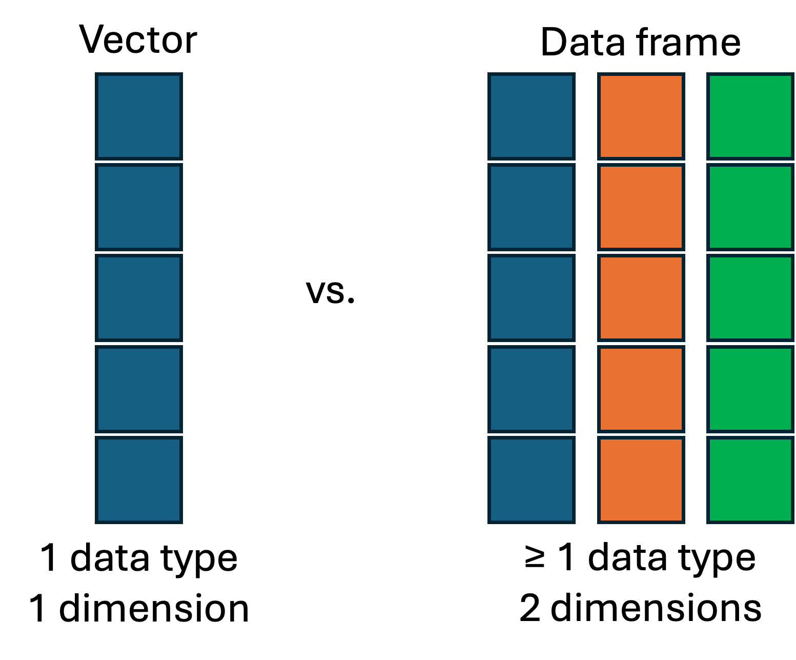
We can easily create a data frame by hand using the data.frame() function and “column_name = column_vector” notation for each column:

birds_df <- data.frame(species = birds,
                       wingspan = wingspans_cm,
                       size = sizes_cm,
                       n_eggs = c(2, 2, 7, 4))

birds_df

      species wingspan  size n_eggs
1 hummingbird     11.8  7.62      2
2  bald_eagle    203.0 90.00      2
3   chickadee     18.2 13.10      7
4    cardinal     27.9 21.80      4

Most often, however, you’ll be reading your data frames from files. And you’ll also want to save your modified data frames.

So let’s practice writing and reading a data frame to and from a “CSV” file — a plain-text, tabular file in which columns are delimited by commas (“Comma-Separated Values” file).

# Write a data frame to CSV format:
write.csv(x = birds_df, file = "sandbox/bird-data.csv", row.names = FALSE)

Curious what the file itself looks like? (Click to expand)

If you want to do the following yourself: next to the R Console, there is tab called Terminal, which will open a Unix shell (!). In there, type the following:

cat sandbox/bird-data.csv

"species","wingspan","size","n_eggs"
"hummingbird",11.8,7.62,2
"bald_eagle",203,90,2
"chickadee",18.2,13.1,7
"cardinal",27.9,21.8,4

Now we read our data frame back in from the file:

birds_df_2 <- read.csv("sandbox/bird-data.csv")

birds_df_2

      species wingspan  size n_eggs
1 hummingbird     11.8  7.62      2
2  bald_eagle    203.0 90.00      2
3   chickadee     18.2 13.10      7
4    cardinal     27.9 21.80      4

9.2 Inspecting a Data Frame

Use str() to look at the “structure” of the data — it tells us the number rows and columns, and for each column, gives information about the data type and shows the first few values:

str(birds_df)

'data.frame':   4 obs. of  4 variables:
 $ species : chr  "hummingbird" "bald_eagle" "chickadee" "cardinal"
 $ wingspan: num  11.8 203 18.2 27.9
 $ size    : num  7.62 90 13.1 21.8
 $ n_eggs  : num  2 2 7 4

For larger data frames, the head() function, which will print the first 6 rows, is also useful (but is of no real use for a tiny data frame like birds_df):

head(birds_df)

      species wingspan  size n_eggs
1 hummingbird     11.8  7.62      2
2  bald_eagle    203.0 90.00      2
3   chickadee     18.2 13.10      7
4    cardinal     27.9 21.80      4

Finally, in RStudio, you can open a data frame in a spreadsheet-like manner by clicking on an object in the “Environment” pane, or equivalently, using View():

View(birds_df)

9.3 Functions to get an overview of data frames

Size:
- nrow() – Number of rows
- ncol() – Number of columns
- dim() – Dimensions: c(number of rows, number of columns)
- length() – For a dataframe: number of columns. For a vector: number of elements.
Content:
- head() – shows the first 6 rows
- tail() – shows the last 6 rows
Names:
- names() or colnames() – column names
- rownames() – row names
Summary:
- str() – structure of the object and information about the class, length and content of each column
- summary() – summary statistics for each column

Exercise: Cars

mtcars is an example data frame that is always available in R.

Use head() to print the first 6 rows of the mtcars dataframe.

Click here for the solution

head(mtcars)

                   mpg cyl disp  hp drat    wt  qsec vs am gear carb
Mazda RX4         21.0   6  160 110 3.90 2.620 16.46  0  1    4    4
Mazda RX4 Wag     21.0   6  160 110 3.90 2.875 17.02  0  1    4    4
Datsun 710        22.8   4  108  93 3.85 2.320 18.61  1  1    4    1
Hornet 4 Drive    21.4   6  258 110 3.08 3.215 19.44  1  0    3    1
Hornet Sportabout 18.7   8  360 175 3.15 3.440 17.02  0  0    3    2
Valiant           18.1   6  225 105 2.76 3.460 20.22  1  0    3    1

How many rows and columns does mtcars contain?

Click here for the solution

It contains 32 rows and 11 columns:

dim(mtcars)

[1] 32 11

Or:

nrow(mtcars)

[1] 32

ncol(mtcars)

[1] 11

Get a vector with the column names of mtcars.

Click here for the solution

colnames(mtcars)

 [1] "mpg"  "cyl"  "disp" "hp"   "drat" "wt"   "qsec" "vs"   "am"   "gear"
[11] "carb"

10 Subsetting

10.1 Basic subsetting of data frames and vectors

We can pull out parts of vectors and data frames using square brackets.

Vectors

For example, for vectors:

# Remind ourselves what this vector contains
wingspans_cm

[1]  11.8 203.0  18.2  27.9

# Get the first element
wingspan_cm[1]

[1] 203

# Get the third element
wingspan_cm[3]

[1] NA

You can pull out larger “slices” from the vector by providing vectors of indices:

# Get the first and the third element
wingspan_cm[c(1, 3)]

[1] 203  NA

The : operator gives you a sequence of consecutive values, which you can also using for slicing:

# Get the second through the fourth element
wingspan_cm[2:4]

[1] NA NA NA

Data frames

To subset data frames, we need to provide two values: row and column, with a comma between them.

For example, to get the element in the 1st row, 1st column:

birds_df[1, 1]

[1] "hummingbird"

To get the element in the 2nd row, 3rd column:

birds_df[2, 3]

[1] 90

To get the entire 2nd row, leave the column part blank:

birds_df[2, ]

     species wingspan size n_eggs
2 bald_eagle      203   90      2

And to extract the entire 3rd column, leave the row part blank:

birds_df[, 3]

[1]  7.62 90.00 13.10 21.80

To extract a column, you can also refer to it by name, in multiple ways:

birds_df$size

[1]  7.62 90.00 13.10 21.80

birds_df[, "size"]

[1]  7.62 90.00 13.10 21.80

Exercise: Subsetting

Extract the 1st-3rd rows and the 4th colum from birds_df.

Click here for the solution

birds_df[1:3, 4]

[1] 2 2 7

Or:

birds_df[c(1, 2, 3), 4]

[1] 2 2 7

Use the $ notation to extract the n_eggs column from birds_df.

Click here for the solution

birds_df$n_eggs

[1] 2 2 7 4

11 Miscellaneous

11.1 Missing data

As R was designed to analyze datasets, it includes the concept of missing data (which is uncommon in other programming languages). Missing data are represented as NA (for “Not Available”).

heights <- c(2, 4, 4, NA, 6)

When doing operations on numbers, most functions will return NA if the data you are working with include missing values. It is a safer behavior as otherwise you may overlook that you are dealing with missing data. You can add the argument na.rm=TRUE to calculate the result while ignoring the missing values.

mean(heights)

[1] NA

mean(heights, na.rm = TRUE)

[1] 4

11.2 Packages

The functions that we have been using so far (and many, many more) are available in any R session as soon as you start R (we refer to this functionality as “base R”). However, when doing specialized analyses such as in microbiomics, rather than coding up everything using the basic building blocks in R, we can load add-on code that will allow us to use “high-level” functions specifically geared towards the effective analyses of such data.

This type of add-on code is distributed in R packages. The default repository for R packages is CRAN, and you install CRAN packages with the install.packages() function:

# Don't run this
install.packages("tidyverse")

If you’re doing bioinformatic analyses in R, as we will be doing, you will encounter packages that are not on CRAN but are on “Bioconductor”. To install a package from Bioconductor, use the BiocManager package – for example:

# Don't run this
install.packages("BiocManager")  # Install the BiocManager package
BiocManager::install("dada2")    # Install the dada2 package from Bioconductor

Installation issues at OSC

The installation of some packages is tricky at OSC nowadays, and if you were to try the commands above, they would likely fail. With a bit of extra effort, we can install these packages, but during the workshop, we will be using a custom collection of pre-installed packages.

11.3 Saving your data

Some very brief notes on saving your data in R:

We already saw the use of write.csv() to save data frames, and you can also use one of readr’s writing functions.

To save R objects “as is”, which can be useful when you’re working with complex S4 objects that may have taken a long time to generate, like a phyloseq object, you can use:

# Don't run this

# Save an object:
saveRDS(my_phyloseq_object, "my_phyloseq_object.RDS")

# Load it again in a new R session:
my_phyloseq_object <- readRDS("my_phyloseq_object.RDS")

A general recommendation is to not rely on your R session to keep things around, especially “overnight”. Devise your workflow such that you are always saving important objects and results outside of R, and can always use your R script to restart from where you left off.

Optional: Change a setting to not let R save your Workspace

Along the line of the above, the default behavior of saving and restoring your “Workspace”, which are all the items (objects) that you create during an R session, is bad practice. Instead, you should always recreate your environment from a script and/or saved files with individual pieces of data.

Change the following setting to prevent R from saving your Workspace whenever you close R:

Click Tools (top bar, below your browser’s address bar) > Global Options
In the pop-up window (stay on the General tab), change the settings under the “Workspace” heading to:

11.4 S4 Objects

While the object types we have discussed so far are so-called “S3” objects, we will also be seeing “S4” objects in this workshop. S4 object are commonly used by bioinformatics packages, for instance phyloseq.

In a nutshell, S4 objects allow for complicated, multifaceted datasets (e.g. multiple dataframes with and metadata) to be represented in a single object in a standardized way.

Unlike S3 objects, S4 objects are usually not manipulated by simple assignment with <-, but with specialized functions that are sure to adhere to the strict object definitions.

12 Where to go from here

This document only scratched the surface of R, but it has hopefully provided a good starting point for working with R.

Here are some potential next steps:

Learn about plotting with ggplot2. Start with these two OSU Code Club sessions:
- ggplot part I
- ggplot part II
Learn about data wrangling with tidyverse packages, especially dplyr and tidyr. Start with these two OSU Code Club sessions:
- Introduction to the tidyverse
- Tidyverse 2: More dplyr Data Wrangling

Both of those topics and some other material are also covered in this excellent Carpentries workshop R for Reproducible Scientific Analysis.

If you want to start with a book, I would recommend Wickham & Grolemund’s “R for Data Science”, which is freely available on the web in a really nice format here.

Want to try the tidyverse (includes ggplot2) at OSC?

If you want to try using the tidyverse in RStudio at OSC now, then load it as follows:

.libPaths("/fs/ess/PAS0471/jelmer/R/metabar")
dyn.load("/fs/ess/PAS0471/jelmer/software/GLPK/lib/libglpk.so.40", local = FALSE)
library(tidyverse)

13 Bonus: conditional subsetting

Another common way of subsetting is by using a logical vector of the same length as the original vector: any TRUE will select the element with the same index, while FALSE will not:

wingspans_cm

[1]  11.8 203.0  18.2  27.9

# This will extract the 1st and the 4th element
wingspans_cm[c(TRUE, FALSE, FALSE, TRUE)]

[1] 11.8 27.9

Typically, these logical vectors are not typed by hand, but are the output of other functions or logical tests. For instance, if you wanted to select only the values above 20:

# This will return a logical vector with TRUE for indices that meet the condition
wingspans_cm > 20

[1] FALSE  TRUE FALSE  TRUE

# We can use such a vector to select only the values above 20
wingspans_cm[wingspans_cm > 20]

[1] 203.0  27.9

`==` and `%in%`

You can test for equality with ==:

"chickadee" == "chickadee"

[1] TRUE

# Which element(s) of the birds vector equal "chickadee"
birds == "chickadee"

[1] FALSE FALSE  TRUE FALSE

# Extract the element(s) of the birds vector that equal "chickadee"
birds[birds == "chickadee"]

[1] "chickadee"

If you want to use a search vector with multiple items, use %in% instead:

# Which element(s) of the birds vector match any of the 3 birds on the right-hand side
birds %in% c("chickadee", "hummingbird", "shoebill")

[1]  TRUE FALSE  TRUE FALSE

# Extract those elements
birds[birds %in% c("chickadee", "hummingbird", "shoebill")]

[1] "hummingbird" "chickadee"

Exercise: Conditional subsetting

Given the following inhabitants of a house, and a list of species to keep:

inhabitants <- c("rat", "rat", "dog", "mouse", "cat", "cat")
keep <- c("dog", "cat")

What do you think the following would return? (Test it and see if you were right.)
```
inhabitants %in% keep
```
```
keep %in% inhabitants
```

Click here for the solution

inhabitants %in% keep

[1] FALSE FALSE  TRUE FALSE  TRUE  TRUE

keep %in% inhabitants

[1] TRUE TRUE

Extract the dogs and cats from the inhabitants vector with logical subsetting.

Click here for the solution

inhabitants[inhabitants %in% keep]

[1] "dog" "cat" "cat"

Attribution

This material was modified after material from The Carpentries, especially from this Data Carpentry workshop and this “R for Ecology” workshop.

Footnotes

The placement of these panes and their content can be customized.↩︎
You created this in the shell introduction. If you don’t have it, create it now.↩︎
In RStudio, typing Alt + - will write <- in a single keystroke. You can also use = as assignment, but that symbol can have other meanings, and so I recommend sticking with the <- combination.↩︎
There are also some other restrictions that are beyond the scope of this introduction. For example, there are some names that cannot be used because they are the names of fundamental keywords in R (e.g., if, else, for, see here for a complete list). In general, it’s also best not to use the names of existing functions, even though this is possible.↩︎
Technically, a vector can have a length of 1, so our earlier single numbers were vectors too.↩︎
This is technically a type of data structure.↩︎
Note, that technically, factors are a data structure, but they are more intuitively thought of as a data type↩︎

1 Why R?

Learning Objectives

2 Getting set up

2.1 Start an RStudio session at OSC

2.2 R vs. RStudio

3 Interacting with R

3.1 R as a calculator

3.2 Trying some random things…

4 Getting Organized

4.1 Need for Scripts and RStudio Projects

4.2 Create a new RStudio Project

4.3 Create an R script

4.4 Commenting

5 R objects

5.1 Assigning stuff to objects

5.2 Object names

Exercises: objects and strings

6 Functions

6.1 Using named arguments

7 Getting help

8 Vectors

8.1 Data types in R

8.2 Vectorization!

Exercise: Temperature conversion

8.3 Other data structures in R

9 Data Frames

9.1 Create, write, and read a data frame

9.2 Inspecting a Data Frame

9.3 Functions to get an overview of data frames

Exercise: Cars

10 Subsetting

10.1 Basic subsetting of data frames and vectors

Vectors

Data frames

Exercise: Subsetting

11 Miscellaneous

11.1 Missing data

11.2 Packages

11.3 Saving your data

11.4 S4 Objects

12 Where to go from here

13 Bonus: conditional subsetting

== and %in%

Exercise: Conditional subsetting

Attribution

Footnotes

`==` and `%in%`