# Set the R library to load packages from
.libPaths("/fs/ess/PAS0471/jelmer/R/metabar")
dyn.load("/fs/ess/PAS0471/jelmer/software/GLPK/lib/libglpk.so.40", local = FALSE)Defining a core microbiome
Introduction: The core microbiome
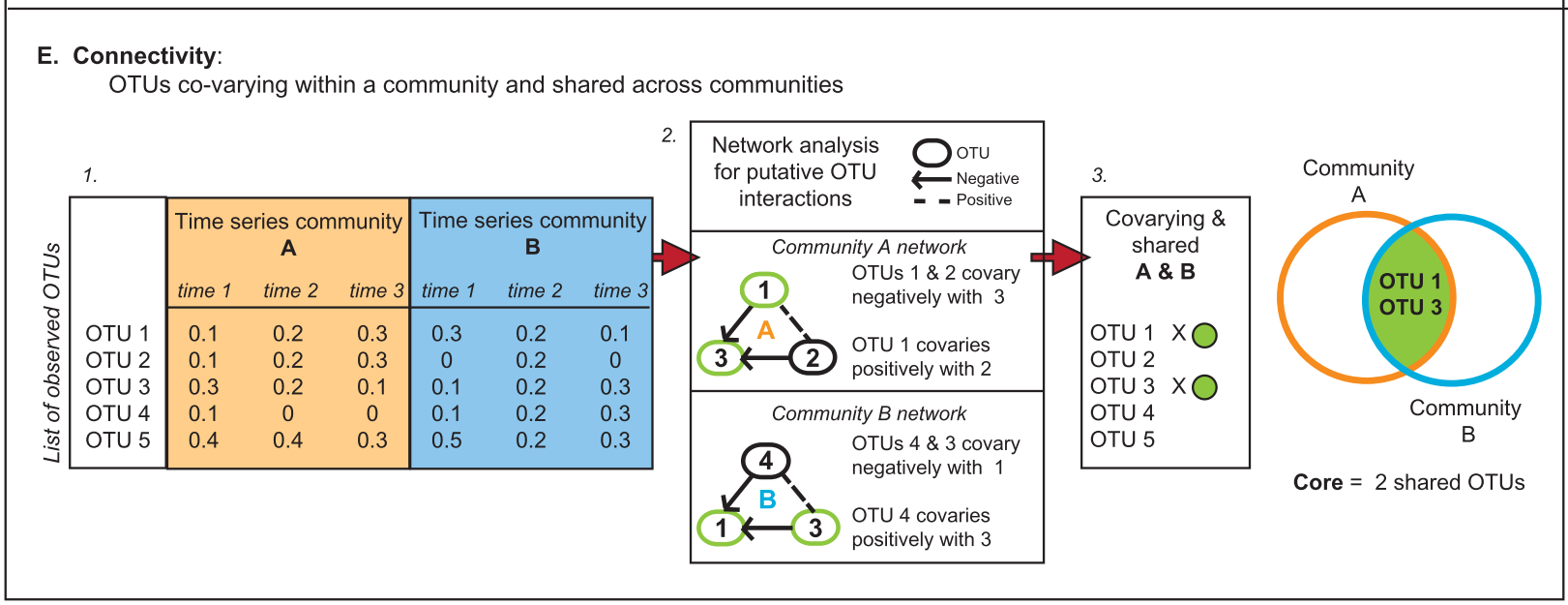
Let’s start understanding what is considered a core microbiome. It comprises the members shared among two or more microbial assemblages associated with a habitat. To define a core microbiome we can consider parameters such as composition (taxonomic membership or community function), phylogeny, persistence, connectivity (biotic/abiotic interactions).
Why is important to define a core microbiome? Important to know the role of key microorganisms and their functions within and across ecosystems. Commonly occurring microorganisms are likely critical to the function of that community. Also, it helps us to define what is a ‘healthy’ community and predict its responses to perturbation.
There are several approaches to define a core microbiome1:
2. Composition (relative abundance)
Accounts for the representation in the community using relative abundance of each OTU/ASV. Dominant and rare members can contribute in different ways to the community. You might focus your analysis in a specific group.

3. Phylogenetic and functional redundancy
Phylogenetic redundancy refers to multiple members from the same lineage present in a microbiome, whereas functional redundancy to members within a microbiome are performing the same functions (e.g. nitrogen fixation). Functional redundancy can help the microbiome buffer disturbance responses.

4. Persistence (temporal and spatial)
Persistence/transience concepts are similar to dominance/rarity. For example: when determining plant-associated microbiomes present across developmental stages.

1 Setting up
If you need to start a new RStudio Server session at OSC or open your RStudio Project, see the box below.
Start an RStudio Server job
- Log in to OSC at https://ondemand.osc.edu.
- Click on
Interactive Apps(top bar) and thenRStudio Server(all the way at the bottom). - Fill out the form as follows:
- Cluster:
Pitzer - R version:
4.3.0 - Project:
PAS2714 - Number of hours:
4 - Node type:
any - Number of cores:
4
- Cluster:
- Click
Launchand once your job has started, clickConnect to RStudio Server.
Open your RStudio Project
- Your RStudio Project at
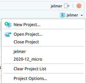
/fs/ess/PAS2714/users/<user>may have automatically opened. You can see whether a Project is open, and if so, which one, in the top-right of your screen (left screenshot below) - If your Project isn’t open, click on the R-in-a-box icon to open it (right screenshot below):

jelmer is open.Your Project name is also your username.
Create a new script (Optional)
Click File > New file > R script, and immediately save the new file (File > Save as) as core.R inside your scripts directory2.
We recommend that you copy-and-paste (or type, if you prefer) code from this webpage into your script and then execute the code. That way, you’ll have a nice record of what you did, exactly.
Load packages
# Load the packages
library(tidyverse)
library(microbiome)
library(phyloseq)
library(ggvenn)
Load the phyloseq object
Read the phyloseq object containing your data:
ps.dataset <- readRDS("results/ps_fulldata/bac22rot_w_ASV.rds")Take a look of your metadata and the variables you want to analyse. We will focus on Rotation.
sample_data(ps.dataset) Year Location Rotation Plot TRT Block Sampling.Date
T22NW102AB 2022 NWARS CS 102AB 2 100 June, 2022
T22NW102C 2022 NWARS CS 102C 7 100 June, 2022
T22NW103AB 2022 NWARS CSW 103AB 3 100 June, 2022
T22NW103C 2022 NWARS CSW 103C 8 100 June, 2022
T22NW201AB 2022 NWARS CSW 201AB 3 200 June, 2022
T22NW201C 2022 NWARS CSW 201C 8 200 June, 2022
T22NW203A 2022 NWARS CS 203A 7 200 June, 2022
T22NW203BC 2022 NWARS CS 203BC 2 200 June, 2022
T22NW305AB 2022 NWARS CS 305AB 2 300 June, 2022
T22NW305C 2022 NWARS CS 305C 7 300 June, 2022
T22NW403A 2022 NWARS CS 403A 7 400 June, 2022
T22NW403BC 2022 NWARS CS 403BC 2 400 June, 2022
T22NW404A 2022 NWARS CSW 404A 8 400 June, 2022
T22NW404BC 2022 NWARS CSW 404BC 3 400 June, 2022
T22W101AB 2022 WARS CS 101AB 2 100 June, 2022
T22W101C 2022 WARS CS 101C 7 100 June, 2022
T22W103AB 2022 WARS CSW 103AB 3 100 June, 2022
T22W103C 2022 WARS CSW 103C 8 100 June, 2022
T22W204A 2022 WARS CSW 204A 8 200 June, 2022
T22W204BC 2022 WARS CSW 204BC 3 200 June, 2022
T22W205A 2022 WARS CS 205A 7 200 June, 2022
T22W205BC 2022 WARS CS 205BC 2 200 June, 2022
T22W303AB 2022 WARS CSW 303AB 3 300 June, 2022
T22W303C 2022 WARS CSW 303C 8 300 June, 2022
T22W304AB 2022 WARS CS 304AB 2 300 June, 2022
T22W304C 2022 WARS CS 304C 7 300 June, 2022
T22W403AB 2022 WARS CS 403AB 2 400 June, 2022
T22W403C 2022 WARS CS 403C 7 400 June, 2022
T22W404A 2022 WARS CSW 404A 8 400 June, 2022
T22W404BC 2022 WARS CSW 404BC 3 400 June, 20222 Approach 1: Composition (relative abundance)
- Transform the ASV count table to compositional data (relative abundance). For that we will use the R package
microbiome(previously installed) with the functiontransform.
ps.dataset.cm <- microbiome::transform(ps.dataset, "compositional")- Determine the core taxa by the variable of interest (Rotation).For this you will subset the data by Rotation variable.
ps.CS <- subset_samples(ps.dataset.cm, Rotation == "CS")
ps.CSW <- subset_samples(ps.dataset.cm, Rotation == "CSW")
Then, get the core taxa using the function core_members from the R package microbiome.
core.taxa.CS <- core_members(ps.CS, detection = 0.001, prevalence = 95/100)
core.taxa.CSW <- core_members(ps.CSW, detection = 0.001, prevalence = 95/100)Detection (limit of detection) will be the minimum relative abundance value at which taxa will be selected. This can be set by the user or determined empirically based on sequencing depth.
Prevalence is the proportion of samples that will be selected given a detection threshold.
Example (click here)
Consider this mock data for relative abundance of Pseudomonas fluorescens in 10 soil microbiome samples:
| Sample | Relative abundance (%) |
|---|---|
| 1 | 0.002 |
| 3 | 0.49 |
| 4 | 7.8 |
| 5 | 12.1 |
| 6 | 0.52 |
| 7 | 0.2 |
| 8 | 0.06 |
| 9 | 9.1 |
| 10 | 0.08 |
Based on detection values, the prevalence will change. Lower detection threshold equals higher prevalence:
| Detection | Prevalence |
|---|---|
| 1 | 3/10 |
| 0.1 | 6/10 |
| 0.01 | 9/10 |
- Create a list with the selected core taxa for both subsets.
cores.list <- list(CS = core.taxa.CS, CSW = core.taxa.CSW)
cores.list #To see the list of core taxa (ASVs) by Rotation
$CS
[1] "ASV_1372" "ASV_1425" "ASV_1426" "ASV_1723" "ASV_1737" "ASV_2316"
[7] "ASV_2440" "ASV_2450" "ASV_2483" "ASV_2545" "ASV_2605" "ASV_2635"
[13] "ASV_2825" "ASV_3076" "ASV_3576" "ASV_3587" "ASV_3592" "ASV_3986"
[19] "ASV_4073" "ASV_4082" "ASV_4242" "ASV_4348" "ASV_4391" "ASV_4478"
[25] "ASV_4504" "ASV_4555" "ASV_4565" "ASV_4642" "ASV_5779" "ASV_5791"
[31] "ASV_6609" "ASV_7160" "ASV_7731" "ASV_7736" "ASV_7822" "ASV_7847"
[37] "ASV_7848" "ASV_8079"
$CSW
[1] "ASV_1367" "ASV_1372" "ASV_1388" "ASV_1425" "ASV_1426" "ASV_1723"
[7] "ASV_1737" "ASV_1863" "ASV_2316" "ASV_2440" "ASV_2450" "ASV_2483"
[13] "ASV_2545" "ASV_2605" "ASV_2619" "ASV_2635" "ASV_2825" "ASV_2896"
[19] "ASV_3076" "ASV_3576" "ASV_3592" "ASV_3898" "ASV_3962" "ASV_3986"
[25] "ASV_4059" "ASV_4073" "ASV_4082" "ASV_4242" "ASV_4391" "ASV_4477"
[31] "ASV_4478" "ASV_4504" "ASV_4521" "ASV_4565" "ASV_4642" "ASV_4654"
[37] "ASV_4655" "ASV_5760" "ASV_5791" "ASV_6609" "ASV_6960" "ASV_7160"
[43] "ASV_7349" "ASV_7731" "ASV_7736" "ASV_7822" "ASV_7848" "ASV_7858"
[49] "ASV_8079"- Get the list of shared taxa from the taxa table of your dataset.
tax.table.ps <- as.data.frame(tax_table(ps.dataset))

shared.taxa <-  core.taxa.CS[core.taxa.CS %in% core.taxa.CSW]
tax <- tax.table.ps[which(row.names(tax.table.ps) %in% shared.taxa ),]- Get the list of unique taxa in Rotation CS.
unique.taxa.CS <-  core.taxa.CS[!core.taxa.CS %in% core.taxa.CSW]
tax.CS <- tax.table.ps[which(row.names(tax.table.ps) %in% unique.taxa.CS),]- Get the list of unique taxa in Rotation CSW.
unique.taxa.CSW <-  core.taxa.CSW[!core.taxa.CSW %in% core.taxa.CS]
tax.CSW <- tax.table.ps[which(row.names(tax.table.ps) %in% unique.taxa.CSW),]- Plot a Venn Diagram.
plot <- ggvenn(cores.list, fill_color = c("#0073C2FF", "#EFC000FF"),
            stroke_size = 0.5, set_name_size = 5, text_size = 5,
            show_percentage = T)
print(plot)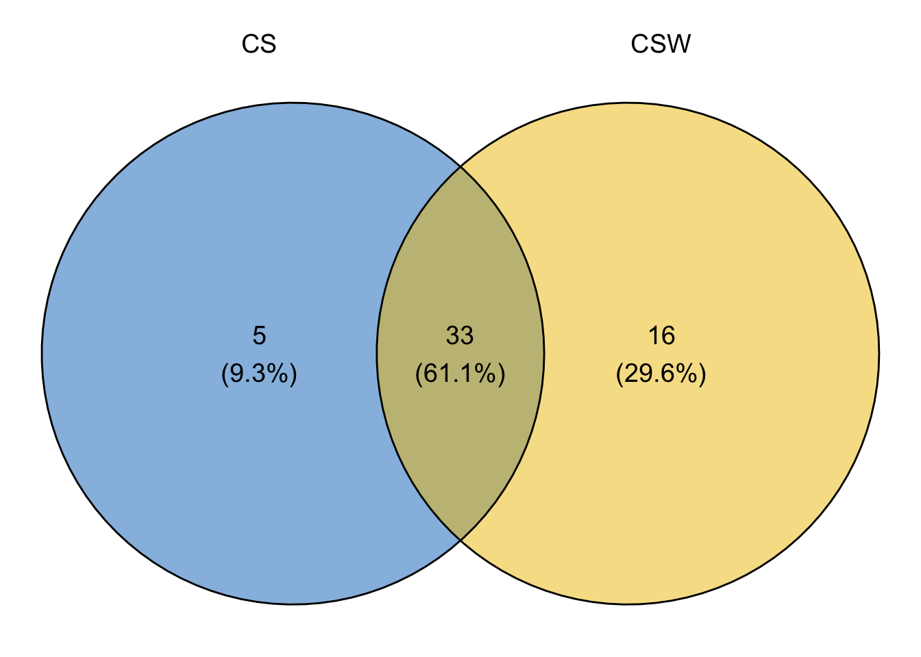
3 Approach 2: Membership and Composition
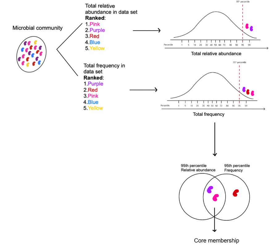
This approach takes into account presence/absence and relative abundance to select shared taxa. The threshold could arbitrary be set but here we will follow the 95th percentile approach3. That means that we will assign core membership to taxa that fell within the 95th percentile of the ranked frequency and ranked relative abundance within the whole data.
Diagram of how the 95th percentile frequency and abundance core taxa were identified. The distribution of total relative abundance and frequency of taxa is assessed and the those ranked within the 95th percentile (top 5%) are selected as core. Figure from Cantoran et al. 2023.
- Create a data frame from the
phyloseqobject.
df <- psmelt(ps.dataset.cm)- Take the total Relative Abundance sum of each genus.
df.RA <- aggregate(df$Abundance, by = list(Genus = df$Genus), FUN=sum)
df.RA <- dplyr::rename(df.RA, TotalRA = `x`)- Determining 95th quantile of the RA data.
quantile.95.abund <- quantile(df.RA$TotalRA, 0.95)- Selecting for genera that fit the 95th cutoff.
taxa.95 <- subset(df.RA, TotalRA >= quantile.95.abund)
taxa.95.genus <- taxa.95$Genus- Determine the frequency 95th cutoff. We go back and use the original phyloseq object and agglomerate the data by Genus tax rank (it could be any tax rank you want e.g., Phylum, Family).
ps.genus <- tax_glom(ps.dataset, "Genus")
ASVs.genus <- otu_table(ps.genus)
df.ASVs.genus <- as.data.frame(ASVs.genus)
rownames(df.ASVs.genus) <- as.data.frame(tax_table(ps.genus))$Genus- Create a table of presence/abundance of ASVs. We will use 1 if present, 0 if not.
df.PA <- 1*((df.ASVs.genus>0)==1)
Occupancy <- rowSums(df.PA)/ncol(df.PA) #Calculate occupancy
df.Freq <- as.data.frame(cbind(df.PA, Occupancy))
df.Freq <- tibble::rownames_to_column(df.Freq, "Genus")- Determining 95th quantile of the presence/abundance table.
quantile.95.freq <- quantile(df.Freq$Occupancy, 0.95)- Select the genera that fit the 95th cutoff.
Freq.95 <- subset(df.Freq, Occupancy >= quantile.95.freq) #select cutoff
Freq.95.genus <- Freq.95$Genus

Quantile.95 <- merge.data.frame(Freq.95, taxa.95, by = "Genus") Use the Freq.95.genus and taxa.95.genus data:
Core.95.list <- list(Frequency = Freq.95.genus, Relative_abundance = taxa.95.genus)

plot.VennD <- ggvenn(Core.95.list,
            stroke_size = 0.5, set_name_size = 3.2, text_size = 3)

print(plot.VennD)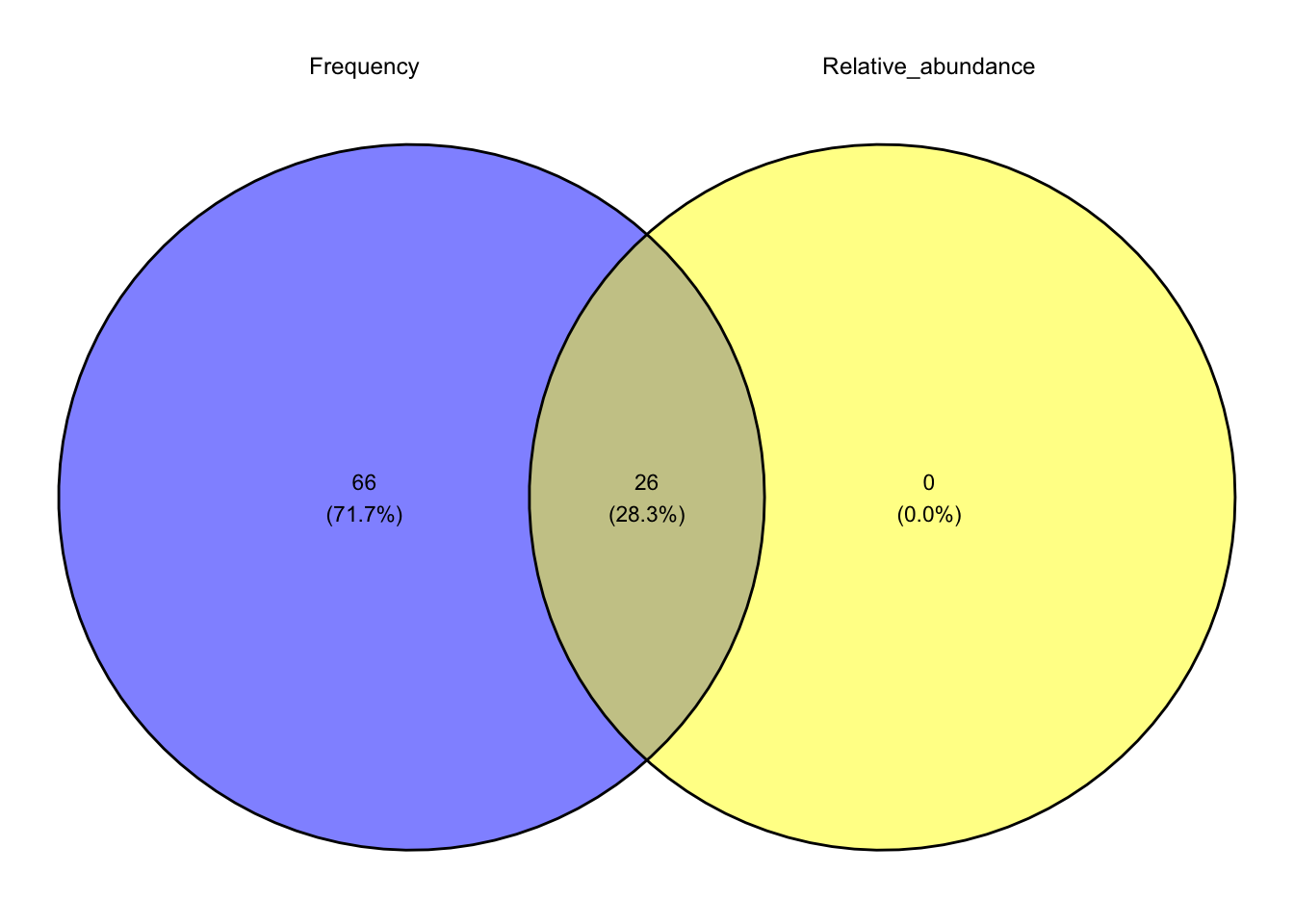
- Get the list of your core taxa based on the 95th percentile.
Core.95.intersect <- Reduce(intersect, Core.95.list)- Subset your original phyloseq object for core taxa.
ps.Core <- subset_taxa(ps.dataset, Genus %in% c(Core.95.intersect))- Fix the relative abundance of the core taxa to continue with the plot.
# Agglomerate taxa by genus level
Core_genera <- tax_glom(ps.Core, taxrank = "Genus", NArm = FALSE)

# Get relative abundance in %
Core_genera.RA <- transform_sample_counts(Core_genera , function(x) 100 * x/sum(x))

#Transform to a data frame
df.Core_genera <- psmelt(Core_genera.RA)- Create a bubble plot. You can customize your plot using
ggplot2package available options.
df.Core_genera %>%
  group_by(Genus, Rotation, Location,) %>%
  summarize(abundance = mean(Abundance)) %>%
  ggplot(aes(Rotation, Genus)) +
  facet_wrap(~Location) +
  geom_point(aes(size = abundance), color = "grey30", fill = "#66A61E",
             alpha = 0.5, shape = 21, stroke = 0.1) +
  scale_size_continuous(range = c(0,8), breaks = c(1, 3, 5, 8, 10),
                        name="Relative\nAbundance (%)") +
  scale_x_discrete(name ="Rotation") +
  theme_bw()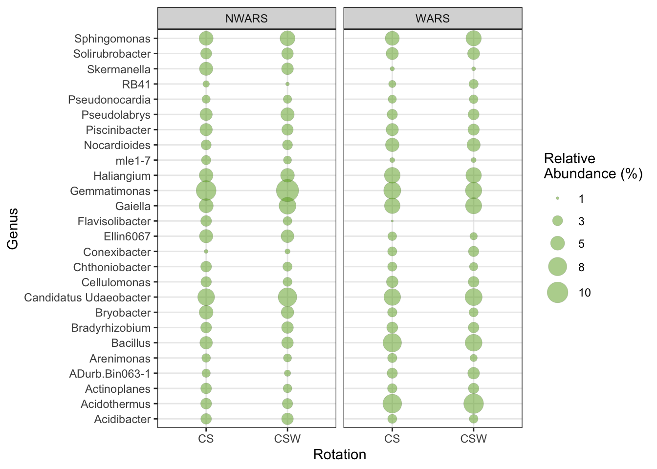
Footnotes
Shade et al. 2012 DOI:https://doi.org/10.1111/j.1462-2920.2011.02585.x↩︎
(you can create that dir in the dialog box if needed↩︎
Cantoran et al. 2023 DOI:https://doi.org/10.1093/femsec/fiad098↩︎

