Homework for the week 4 lab: R basics

Author

Affiliation

Jelmer Poelstra

CFAES Bioinformatics Core, Ohio State University

Published

January 30, 2026

1 Introduction

This homework is intended to get you introduce you to the basics of R & RStudio, because the week 4 lab will involve using R for RNA-Seq data analysis. As such, this is mostly intended for those with little to no experience with R, but:

Even if you’ve worked with R before, at least glance over all material to make sure you’re familiar with all of it
Everyone should install several R packages in RStudio at the Ohio Supercomputer Center (OSC) – section 8

If you run out of steam or time while trying to do this homework, you can stop after section 10 (R objects). But we will see examples of the topics covered in section 11-13 in the week 4 lab.

If you run into any issues when going through this material, or have questions, don’t hesitate to email Jelmer.

1.1 Learning objectives

In this session, you will learn:

The RStudio layout and the functions of the different panes and tabs
The basics of interacting with R by using R as a calculator
Creating objects in R, and assigning values/data to them
Calling functions
Getting help
Installing and loading packages
Data structures like vectors and data frames
The basics of the tidyverse packages, including piping with |>

2 R and RStudio

2.1 Why use R?

After initial processing high-throughput sequencing (HTS) data such as with command-line tools in the Unix shell, you’ll often want to perform statistical analysis and visualization of the results. The R language is probably the best environment for this.

On top of that, R is a great all-round tool to perform the analysis and visualization of any kind of data — together with Python, it is the leading data science language. Because it is free, open-source, cross-platform, and works with code rather than a graphical user interface (GUI), using R also helps with reproducibility of your research.

2.2 R vs. RStudio

To run R, all you need is the R program with its “console” where you type commands. However, we will be running R inside a fancy editor called RStudio, which makes working with R much more pleasant!

3 Start an RStudio session at OSC

While you can install and use R and RStudio on your own computer, for this course, you will use RStudio at OSC: you can run a version of RStudio at OSC within your browser by starting an Interactive App through OnDemand.

Log in to OSC’s OnDemand portal at https://ondemand.osc.edu
In the blue top bar, select Interactive Apps and at the bottom, click RStudio Server
Fill out the form as follows:
- Cluster: cardinal
- R version: 4.4.0
- Project: PAS2880
- Number of hours: 3
- Node type: any
- Number of cores: 1
Click Launch
Click the Connect to RStudio Server button once it appears

If you run out of time for this session, or want to spread this homework across multiple short sessions: you can always start a new session for as many sessions as you want, and you can modify the number of hours in the form as you see fit.

4 Orienting to RStudio

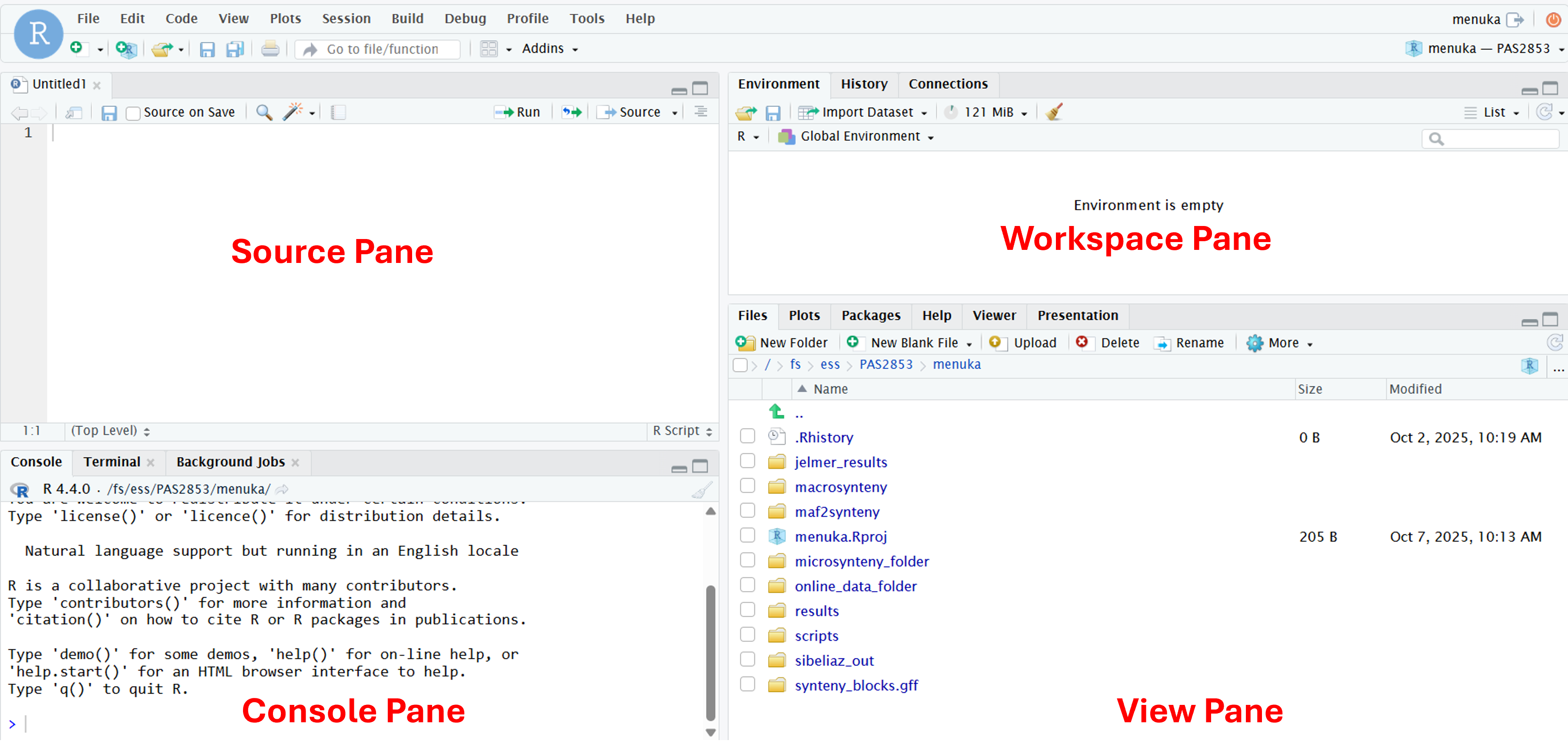
RStudio is divided into four panes, each of which have multiple tabs – we will highlight the most important ones here:

Top left: Source (or Editor)
Here, you can open and edit text documents like scripts (May be missing if you don’t have any documents open – if so, we’ll make it appear later)
Bottom left: Console
Here, you can type and execute R code
Top right: Workspace
The default Environment tab shows you what you have loaded in your R environment
Bottom right: View
The default tab in this pane is “Files”, a file explorer. Also commonly used are e.g. Plots, where plots appear, and Help, for help info.

A screenshot showing the four main RStudio panes

5 R basics

5.1 R as calculator

To get some familiarity with working in R, you will start by simply using R as calculator. Type 5 + 5 in the console and press Enter:

5 + 5

[1] 10

R will print the result of the calculation, 10. The result is prefaced by [1], which is simply an index/count of output items – this can be helpful when many items are printed.

A couple more examples:

# Multiplication
6 * 8

[1] 48

# Division
40 / 5

[1] 8

This code will work with (like shown above) or without spaces between numbers and around operators like +. However, it is good practice to leave space between the number to improve the readability of your code.

5.2 The R prompt

The > sign in your console is the R prompt, indicating that that R is ready for you to type something. In other words, this is equivalent to the $ Shell prompt you’ve seen in the week 3 lab.

When you are not seeing the prompt, R is either busy (because you asked it to do a longer-running computation) or waiting for you to complete an incomplete command. If you notice that your prompt turned into a +, you typed an incomplete command – for example:

10 /

You can either try to finish the command or abort it by pressing Ctrl+C or Esc – go ahead and practice the latter now to get your prompt back after the above command.

Adding comments to your code

Comments in R are also just like in the Unix shell: you can use # signs to comment your code, both inline and on separate lines:

# This line is entirely ignored by R
10 / 5  # This line contains code but everything after the '#' is ignored

[1] 2

5.3 Comparing things

In R, you can use comparison operators to compare numbers. When you do this, R will return either FALSE or TRUE (the so-called logical data type). For example:

Greater than and less than:
```
8 > 3
```
```
[1] TRUE
```
```
2 < 1
```
```
[1] FALSE
```
Equal to or not equal to – note that you need to use two equals signs == for the former:
```
7 == 7
```
```
[1] TRUE
```
```
# The exclamation mark in general is a "negator"
10 != 5
```
```
[1] TRUE
```

You will commonly use these types of comparisons to check and subset/filter your data.

6 Functions in R

To do almost anything in R, you will use “functions”, which are the equivalent of Unix commands. R has over 3,000 functions that serve many different purposes.

6.1 Basics of functions

You can recognize function calls by the parentheses. For example:

The equivalent to the Shell’s pwd is getwd() for “get working dir”:

# You will see a different output depending on your working directory
getwd()

/users/PAS2880/jelmer

Inside those parentheses, you can provide arguments to a function¹. For example, using setwd(), the equivalent to the Shell’s cd, to set your working dir, the argument is the file path to set as working dir:
```
setwd("/fs/scratch/PAS2880/ENT6703")
```
Note that unlike in the Shell, you need to quote ("..") the file path! This is because in R, anything non-numeric that is not quoted is supposed to be a pre-existing “object” – more on those in a bit.

6.2 Function arguments

Consider the example below, where you pass the argument 6.53 to the function round():

round(6.53)

[1] 7

In most functions, including round(), arguments have names that can be used. The argument to round(), which represents the number to be rounded, has the name x, so you can also use:

# This is equivalent to the above:
round(x = 6.53)

[1] 7

Naming arguments is helpful in particular to avoid confusion when you pass multiple arguments to a function. For example, round() accepts a second argument, which is the number of digits to round to:

round(x = 6.53, digits = 1)

[1] 6.5

You could choose not to name these arguments, but that is not as easy to understand for someone reading your code – such as yourself two months later! ²

You can usually see which arguments a function takes by pausing after your type the function and its parenthesis, e.g. round():

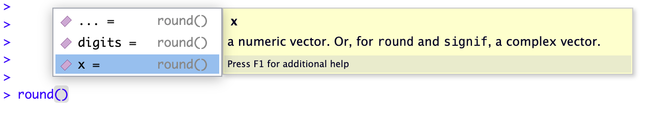
Below, you’ll also learn about ways to get more extensive help information about a function.

7 R Help: `help()` and `?`

So how can you know what a function does, and which arguments it takes? The help() function and ? help operator in R offer access to documentation pages for R functions – as well as built-in data sets and other objects. For example:

?getwd

The output should appear in the Help tab of the bottom-left panel in RStudio and look something like this:

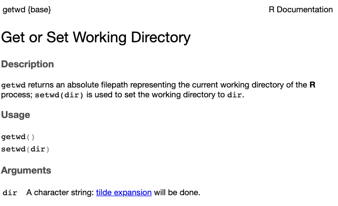
The R help output for the `getwd()` function

You can also search for Help pages in that same RStudio Help tab.

8 R packages

R packages are basically add-ons or extensions to the functionality of the R language. These need to installed and loaded:

The function install.packages() installs an R package. This is a one-time operation – you won’t need to reinstall a package when you start a new R session later³.
The function library() will load an R package in your current R session. Every time you want to use a package in R, you need to load it – just like everytime you want to use MS Word on your computer, you need to open it.

To practice with this, you will now install several packages you’ll need in next week’s lab. Note that:

Unfortunately, on OSC, packages installation can take a while. Especially for large packages like these, so please be patient⁴.
A lot of messages may be printed to the console when installation is ongoing. Installation of a package is done when you get your prompt back. Unless you see clear messages that include words like “Error” and “Failed”, it should have succeeded (“Warning”s are typically okay).
Besides install.packages(), you’ll also use the BiocManager::install() function from to install some packages from Bioconductor, a separate repository that hosts many bioinformatics/omics-related R packages.

# Run these lines one-by-one to install the needed packages --
# First, the tidyverse, which is discussed at the end of this homework
install.packages("tidyverse")

# [... lots of output ...]
# [The last lines should look something like this:]
** testing if installed package can be loaded from temporary location
** testing if installed package can be loaded from final location
** testing if installed package keeps a record of temporary installation path
* DONE (tidyverse)

The downloaded source packages are in
    ‘/tmp/RtmpS4n222/downloaded_packages’

# This is needed to in turn install the next two packages:
# (Should take <1 minute to install)
install.packages("BiocManager")

# We will use this for differential expression analysis:
# (May take 5-10 minutes to install)
BiocManager::install("DESeq2")

# We will use this to create a data visualization called a volcano plot:
# (Should take <1 minute to install)
BiocManager::install("EnhancedVolcano")

Test that you can load the packages – see the expected output below:

library(EnhancedVolcano)

Loading required package: ggplot2

Loading required package: ggrepel

library(DESeq2)

Click here to see the expected output when loading the ‘DESeq2’ package

library(DESeq2)

Loading required package: S4Vectors

Loading required package: stats4

Loading required package: BiocGenerics

Loading required package: generics


Attaching package: 'generics'

The following objects are masked from 'package:base':

    as.difftime, as.factor, as.ordered, intersect, is.element, setdiff,
    setequal, union


Attaching package: 'BiocGenerics'

The following objects are masked from 'package:stats':

    IQR, mad, sd, var, xtabs

The following objects are masked from 'package:base':

    anyDuplicated, aperm, append, as.data.frame, basename, cbind,
    colnames, dirname, do.call, duplicated, eval, evalq, Filter, Find,
    get, grep, grepl, is.unsorted, lapply, Map, mapply, match, mget,
    order, paste, pmax, pmax.int, pmin, pmin.int, Position, rank,
    rbind, Reduce, rownames, sapply, saveRDS, table, tapply, unique,
    unsplit, which.max, which.min


Attaching package: 'S4Vectors'

The following object is masked from 'package:utils':

    findMatches

The following objects are masked from 'package:base':

    expand.grid, I, unname

Loading required package: IRanges

Loading required package: GenomicRanges

Loading required package: GenomeInfoDb

Loading required package: SummarizedExperiment

Loading required package: MatrixGenerics

Loading required package: matrixStats


Attaching package: 'MatrixGenerics'

The following objects are masked from 'package:matrixStats':

    colAlls, colAnyNAs, colAnys, colAvgsPerRowSet, colCollapse,
    colCounts, colCummaxs, colCummins, colCumprods, colCumsums,
    colDiffs, colIQRDiffs, colIQRs, colLogSumExps, colMadDiffs,
    colMads, colMaxs, colMeans2, colMedians, colMins, colOrderStats,
    colProds, colQuantiles, colRanges, colRanks, colSdDiffs, colSds,
    colSums2, colTabulates, colVarDiffs, colVars, colWeightedMads,
    colWeightedMeans, colWeightedMedians, colWeightedSds,
    colWeightedVars, rowAlls, rowAnyNAs, rowAnys, rowAvgsPerColSet,
    rowCollapse, rowCounts, rowCummaxs, rowCummins, rowCumprods,
    rowCumsums, rowDiffs, rowIQRDiffs, rowIQRs, rowLogSumExps,
    rowMadDiffs, rowMads, rowMaxs, rowMeans2, rowMedians, rowMins,
    rowOrderStats, rowProds, rowQuantiles, rowRanges, rowRanks,
    rowSdDiffs, rowSds, rowSums2, rowTabulates, rowVarDiffs, rowVars,
    rowWeightedMads, rowWeightedMeans, rowWeightedMedians,
    rowWeightedSds, rowWeightedVars

Loading required package: Biobase

Welcome to Bioconductor

    Vignettes contain introductory material; view with
    'browseVignettes()'. To cite Bioconductor, see
    'citation("Biobase")', and for packages 'citation("pkgname")'.


Attaching package: 'Biobase'

The following object is masked from 'package:MatrixGenerics':

    rowMedians

The following objects are masked from 'package:matrixStats':

    anyMissing, rowMedians

library(tidyverse)

── Attaching core tidyverse packages ──────────────────────── tidyverse 2.0.0 ──
✔ dplyr     1.1.4     ✔ readr     2.1.5
✔ forcats   1.0.1     ✔ stringr   1.5.2
✔ lubridate 1.9.4     ✔ tibble    3.3.0
✔ purrr     1.1.0     ✔ tidyr     1.3.1
── Conflicts ────────────────────────────────────────── tidyverse_conflicts() ──
✖ lubridate::%within%()    masks IRanges::%within%()
✖ dplyr::collapse()        masks IRanges::collapse()
✖ dplyr::combine()         masks Biobase::combine(), BiocGenerics::combine()
✖ dplyr::count()           masks matrixStats::count()
✖ dplyr::desc()            masks IRanges::desc()
✖ tidyr::expand()          masks S4Vectors::expand()
✖ dplyr::filter()          masks stats::filter()
✖ dplyr::first()           masks S4Vectors::first()
✖ dplyr::lag()             masks stats::lag()
✖ BiocGenerics::Position() masks ggplot2::Position(), base::Position()
✖ purrr::reduce()          masks GenomicRanges::reduce(), IRanges::reduce()
✖ dplyr::rename()          masks S4Vectors::rename()
✖ lubridate::second()      masks S4Vectors::second()
✖ lubridate::second<-()    masks S4Vectors::second<-()
✖ dplyr::slice()           masks IRanges::slice()
ℹ Use the conflicted package (<http://conflicted.r-lib.org/>) to force all conflicts to become errors

For now, don’t worry about the “conflict” warnings shown above.

9 R scripts

You should mostly write and save your R code in so-called “R scripts”, which are text files with R code. This helps keep track of what you’ve been doing and makes it easier to modify and rerun things.

Create and open a new R script by clicking File (top menu bar) > New File > R Script.
Save this new script right away by clicking File > Save As. In the dialog box, you can save it right in the suggested folder, or you can make a new folder for this course. Regardless, save the script as homework.R (the extension for R scripts is .R).

But isn’t a hassle to have to copy-paste code from a script to the console? Well, RStudio makes this pretty easy: to execute code from the script in the the console, press Ctrl + Enter on Windows, or Cmd + Return on a Mac. Practice that after typing the following in the script:

# Type this in the script, then run it with Ctrl + Enter (or Cmd + Return)
5 + 5

[1] 10

10 R objects

Objects are a key concept in R and other programming languages. They can store data and values that you can manipulate and analyze. It takes some time to get used to working with -and conceptualizing- objects, but you will get the hang of it with some practice.

10.1 Assigning stuff to objects

You can assign one or more values to a so-called “object” with the assignment operator <-:

# Assign the value 250 the object 'length_cm':
length_cm <- 250

# Now print the value of this object to screen simply by typing its name:
length_cm

[1] 250

Another example:

conversion <- 2.54
conversion

[1] 2.54

Importantly, you can use objects as if you had typed their values directly:

length_cm / conversion

[1] 98.4252

10.2 Object names

Some pointers on object names:

Because R is case sensitive, length_inch is different from Length_Inch!
An object name cannot contain spaces — so for readability, you can for example separate words e.g. using underscores, as in length_cm.
Object names can contain but cannot start with a number: x2 is valid but 2x is not.
Make object names descriptive yet not too long — this is not always easy!

Exercise: Assigning objects in R

Assign the value 20 to the object num_1, and the value 15 to num_2
Click to see the solution
```
num_1 <- 20
num_2 <- 15
```
Compute the sum of num_1 and num_2
Click to see the solution
```
num_1 + num_2
```
```
[1] 35
```
Assign the result of num_1 minus num_2 to a new object called difference. What is the value of difference?
Click to see a solution
```
difference <- num_1 - num_2
difference
```
```
[1] 5
```
Which of the following are valid object names in R?
1. 2nd_value
2. value_2
3. total value
4. TotalValue
Click to see a solution

The valid object names are:
1. value_2
2. TotalValue
Object names cannot start with a number and cannot contain spaces (so a and c options are invalid).

11 Vectors

R has several so-called “data structures”, distinct object types to store different kinds of data. The most basic of these is the vector, which is simply a collections of one or more items.

11.1 Creating vectors

You’ve already created a few vectors, as the single-item num_1 etc. objects above were vectors! So let’s see something new here: a common way to make vectors with multiple elements is with the c (combine) function:

# longer_vector will contain 3 items:
longer_vector <- c(10, 20, 30)
longer_vector

[1] 10 20 30

For ranges of integers (whole numbers), you can also use the colon operator :

# longer_vector will contain 10 items:
sequence_vector <- 1:10
sequence_vector

 [1]  1  2  3  4  5  6  7  8  9 10

11.2 Exploring vectors

R has many functions that provide information about vectors and other types of objects, such as to get the number of items, or the mean or sum of the values of these items⁵:

# Get the number of items:
length(longer_vector)

[1] 3

# Get the the mean (average) across all elements:
mean(longer_vector)

[1] 20

# Get the sum of all elements:
sum(longer_vector)

[1] 60

11.3 Extracting elements from vectors

You can extract items from objects like vectors using “bracket notation” – get the second item with [2]:

longer_vector[2]

[1] 20

Or get the first and third items with [c(1, 3)]:

longer_vector[c(1, 3)]

[1] 10 30

12 Data frames

Data frames are a key R data structure that contain tabular data – data organized in rows and columns, similar to spreadsheets. An example is the iris data frame that comes shipped with R, which contains measurements for three different species of iris.

You can take a look at the first few rows of this data frame using the head() function:

# Note that each row represents one individual iris flower:
head(iris)

  Sepal.Length Sepal.Width Petal.Length Petal.Width Species
1          5.1         3.5          1.4         0.2  setosa
2          4.9         3.0          1.4         0.2  setosa
3          4.7         3.2          1.3         0.2  setosa
4          4.6         3.1          1.5         0.2  setosa
5          5.0         3.6          1.4         0.2  setosa
6          5.4         3.9          1.7         0.4  setosa

How many columns does this data frame have?(Click for the solution)

This data frame has 5 columns: Sepal.Length, Sepal.Width, Petal.Length, Petal.Width, and Species. The 1 to 6 on the left are the row names, in this case a simple numbering of the rows.

For data frames, the View() function is also neat, as it opens the data frame in a spreadsheet-like viewer – try it!

View(iris)

You can extract individual columns from a data frame using the $ operator:

# Extract the 'Sepal.Width' column from the 'iris' data frame:
iris$Sepal.Width

  [1] 3.5 3.0 3.2 3.1 3.6 3.9 3.4 3.4 2.9 3.1 3.7 3.4 3.0 3.0 4.0 4.4 3.9 3.5
 [19] 3.8 3.8 3.4 3.7 3.6 3.3 3.4 3.0 3.4 3.5 3.4 3.2 3.1 3.4 4.1 4.2 3.1 3.2
 [37] 3.5 3.6 3.0 3.4 3.5 2.3 3.2 3.5 3.8 3.0 3.8 3.2 3.7 3.3 3.2 3.2 3.1 2.3
 [55] 2.8 2.8 3.3 2.4 2.9 2.7 2.0 3.0 2.2 2.9 2.9 3.1 3.0 2.7 2.2 2.5 3.2 2.8
 [73] 2.5 2.8 2.9 3.0 2.8 3.0 2.9 2.6 2.4 2.4 2.7 2.7 3.0 3.4 3.1 2.3 3.0 2.5
 [91] 2.6 3.0 2.6 2.3 2.7 3.0 2.9 2.9 2.5 2.8 3.3 2.7 3.0 2.9 3.0 3.0 2.5 2.9
[109] 2.5 3.6 3.2 2.7 3.0 2.5 2.8 3.2 3.0 3.8 2.6 2.2 3.2 2.8 2.8 2.7 3.3 3.2
[127] 2.8 3.0 2.8 3.0 2.8 3.8 2.8 2.8 2.6 3.0 3.4 3.1 3.0 3.1 3.1 3.1 2.7 3.2
[145] 3.3 3.0 2.5 3.0 3.4 3.0

This kind of operation will return a vector – which can be subsetted as well:

# Extract the 2nd to 5th items from the 'Sepal.Width' column:
iris$Sepal.Width[2:5]

[1] 3.0 3.2 3.1 3.6

13 A brief introduction to the tidyverse and pipes

Finally, you’ll learn a little about a versatile family of R packages designed for data science called the “tidyverse”. The tidyverse is quite large and includes the famous ggplot2 package for data visualization – we’ll barely scratch the surface here, but this should already give you some useful tools.

13.1 `read_tsv()` to read tabular data

The read_tsv() function reads a TSV (Tab-Separated Values) file into a dataframe, taking the path to the file as its main argument – here, read the sample metadata file used in next week’s lab:

meta <- read_tsv("/fs/scratch/PAS2880/ENT6703/data/meta/metadata.tsv")

Rows: 22 Columns: 3
── Column specification ────────────────────────────────────────────────────────
Delimiter: "\t"
chr (2): sample_id, treatment
dbl (1): dpi

ℹ Use `spec()` to retrieve the full column specification for this data.
ℹ Specify the column types or set `show_col_types = FALSE` to quiet this message.

Some info about how it interpreted the data is printed, especially about the data types of different columns (see the box below). Take a look at the resulting data frame meta:

meta

# A tibble: 22 × 3
   sample_id     dpi treatment  
   <chr>       <dbl> <chr>      
 1 ERR10802864     1 cathemerium
 2 ERR10802867     1 cathemerium
 3 ERR10802870     1 cathemerium
 4 ERR10802866     1 control    
 5 ERR10802869     1 control    
 6 ERR10802863     1 control    
 7 ERR10802871     1 relictum   
 8 ERR10802874     1 relictum   
 9 ERR10802865     1 relictum   
10 ERR10802868     1 relictum   
# ℹ 12 more rows

Tibble??

The data frame is a so-called “tibble”, as the top of the output above says. This is a modern take on data frames provided by the tidyverse. Tibbles behave mostly like data frames, but have some nice features mostly in the way they are printed to screen.

For example, the “data types” of columns are shown at the top of the output above, where chr means character (text data) and dbl means double (numeric data; other data types exist as well).

13.2 `select()` to pick columns

The select() function subsets a data frame by including/excluding certain columns. By default, it only includes the columns you specify:

select(.data = meta, sample_id, treatment)

# A tibble: 22 × 2
   sample_id   treatment  
   <chr>       <chr>      
 1 ERR10802864 cathemerium
 2 ERR10802867 cathemerium
 3 ERR10802870 cathemerium
 4 ERR10802866 control    
 5 ERR10802869 control    
 6 ERR10802863 control    
 7 ERR10802871 relictum   
 8 ERR10802874 relictum   
 9 ERR10802865 relictum   
10 ERR10802868 relictum   
# ℹ 12 more rows

Above, the first argument was the data frame, whereas the other arguments were the (unquoted!) names of columns to be kept. The output is a new, modified dataframe. In the example above, this data frame was simply printed to the screen – but as you’ll see later, it can be stored too.

13.3 `filter()` to pick rows (observations)

The filter() function outputs only those rows that satisfy one or more conditions, similar to Filter functionality in Excel. For example, to only keep rows for the 1 timepoint:

filter(.data = meta, dpi == 1)

# A tibble: 10 × 3
   sample_id     dpi treatment  
   <chr>       <dbl> <chr>      
 1 ERR10802864     1 cathemerium
 2 ERR10802867     1 cathemerium
 3 ERR10802870     1 cathemerium
 4 ERR10802866     1 control    
 5 ERR10802869     1 control    
 6 ERR10802863     1 control    
 7 ERR10802871     1 relictum   
 8 ERR10802874     1 relictum   
 9 ERR10802865     1 relictum   
10 ERR10802868     1 relictum

13.4 The pipe (`|>`)

It’s common to want to use several consecutive functions to wrangle a dataframe into the format you want. For example, you may want to first select() one or more columns, then filter() the resulting dataframe. You could do that as follows:

meta_sel <- select(.data = meta, sample_id, dpi)
filter(.data = meta_sel, dpi == 1)

# A tibble: 10 × 2
   sample_id     dpi
   <chr>       <dbl>
 1 ERR10802864     1
 2 ERR10802867     1
 3 ERR10802870     1
 4 ERR10802866     1
 5 ERR10802869     1
 6 ERR10802863     1
 7 ERR10802871     1
 8 ERR10802874     1
 9 ERR10802865     1
10 ERR10802868     1

You could go on along these lines, successively creating new objects that you then use for the next step. But there is a more elegant way of dong this, directly sending (“piping”) output from one function into the next function with the pipe operator |> (a vertical bar | followed by a greater-than sign >).

Let’s start by seeing a reformulation of the code above with pipes:

meta |>
  select(sample_id, dpi) |>
  filter(dpi == 1)

# A tibble: 10 × 2
   sample_id     dpi
   <chr>       <dbl>
 1 ERR10802864     1
 2 ERR10802867     1
 3 ERR10802870     1
 4 ERR10802866     1
 5 ERR10802869     1
 6 ERR10802863     1
 7 ERR10802871     1
 8 ERR10802874     1
 9 ERR10802865     1
10 ERR10802868     1

What happened here? You took the meta data frame, sent (“piped”) it into the select() function, whose output in turn was piped into the filter() function. You can think of the pipe as “then”: take meta, then select, then rename.

When using the pipe, you no longer specify the input with the .data argument, because the function now gets its input data via the pipe. Using pipes involves less typing and is more readable than successive assignments.

For code readability, start a new line after every pipe |> and indent subsequent lines, as seen above.

Exercise: Tidyverse functions and pipes

Use a “pipeline” like above to output a data frame with two columns (sample_id and treatment) only for the cathemerium treatment. How many rows does your output data frame have?

Click for the solution

meta |>
  select(sample_id, treatment) |>
  filter(treatment == "cathemerium")

# A tibble: 7 × 2
  sample_id   treatment  
  <chr>       <chr>      
1 ERR10802864 cathemerium
2 ERR10802867 cathemerium
3 ERR10802870 cathemerium
4 ERR10802882 cathemerium
5 ERR10802875 cathemerium
6 ERR10802879 cathemerium
7 ERR10802883 cathemerium

The output data frame has 7 rows and 2 columns: note that “7 x 2” is helpfully shown at the top of the output in the console.

Optional: Using the pipe keyboard shortcut (Click to expand)

The following RStudio keyboard shortcut will insert a pipe symbol: Ctrl/Cmd + Shift + M.

However, by default this (still) inserts an older pipe symbol, %>%. To make RStudio insert the |> pipe symbol with this keyboard shortcut:

Click Tools > Global Options > Code tab on the right
Check the box “Use native pipe operator” as shown below
Click OK at the bottom of the options dialog box to apply the change and close the box.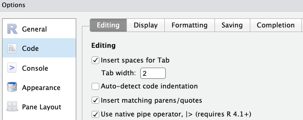

Footnotes

In R, there is no distinction between options and arguments like with Shell commands.↩︎
And unlike unnamed arguments, named arguments can be presented in any order you like.↩︎
This also applies at OSC↩︎
This should be much faster on your own computer.↩︎
The latter two only with numeric vectors - as vectors can also contain text.↩︎

1 Introduction

1.1 Learning objectives

2 R and RStudio

2.1 Why use R?

2.2 R vs. RStudio

3 Start an RStudio session at OSC

4 Orienting to RStudio

5 R basics

5.1 R as calculator

5.2 The R prompt

5.3 Comparing things

6 Functions in R

6.1 Basics of functions

6.2 Function arguments

7 R Help: help() and ?

8 R packages

9 R scripts

10 R objects

10.1 Assigning stuff to objects

10.2 Object names

Exercise: Assigning objects in R

11 Vectors

11.1 Creating vectors

11.2 Exploring vectors

11.3 Extracting elements from vectors

12 Data frames

13 A brief introduction to the tidyverse and pipes

13.1 read_tsv() to read tabular data

13.2 select() to pick columns

13.3 filter() to pick rows (observations)

13.4 The pipe (|>)

Exercise: Tidyverse functions and pipes

Footnotes

7 R Help: `help()` and `?`

13.1 `read_tsv()` to read tabular data

13.2 `select()` to pick columns

13.3 `filter()` to pick rows (observations)

13.4 The pipe (`|>`)