Transcriptomics with RNA-Seq
2026-02-05
Gene expression is functionally important
Considering:
That protein production tells us about the activity of biological functions,
and the molecular mechanisms underlying those functionsThat it is easier to measure transcript (mRNA) than protein abundance
The central dogma

… gene expression can be used as a proxy for protein expression to make functional inferences
Caveat: the correlation between mRNA and protein levels is rather imperfect –
see e.g. Ponomarenko et al. (2023).
What is RNA-Seq?
To estimate gene expression levels genome-wide, RNA-Seq takes a brute-force approach by randomly sequencing of millions of RNA fragments per sample
The resulting reads can be assigned a gene of origin,
and the core idea is that a gene’s read count reflects that gene’s expression level
How can we tell which gene each read originates from?
Most commonly by aligning the reads to a reference genome.What is RNA-Seq?
To estimate gene expression levels genome-wide, RNA-Seq takes a brute-force approach by randomly sequencing of millions of RNA fragments per sample
The resulting reads can be assigned a gene of origin,
and the core idea is that a gene’s read count reflects that gene’s expression level
RNA-Seq is a very widely used technique —
it constitutes the most common usage of high-throughput sequencing
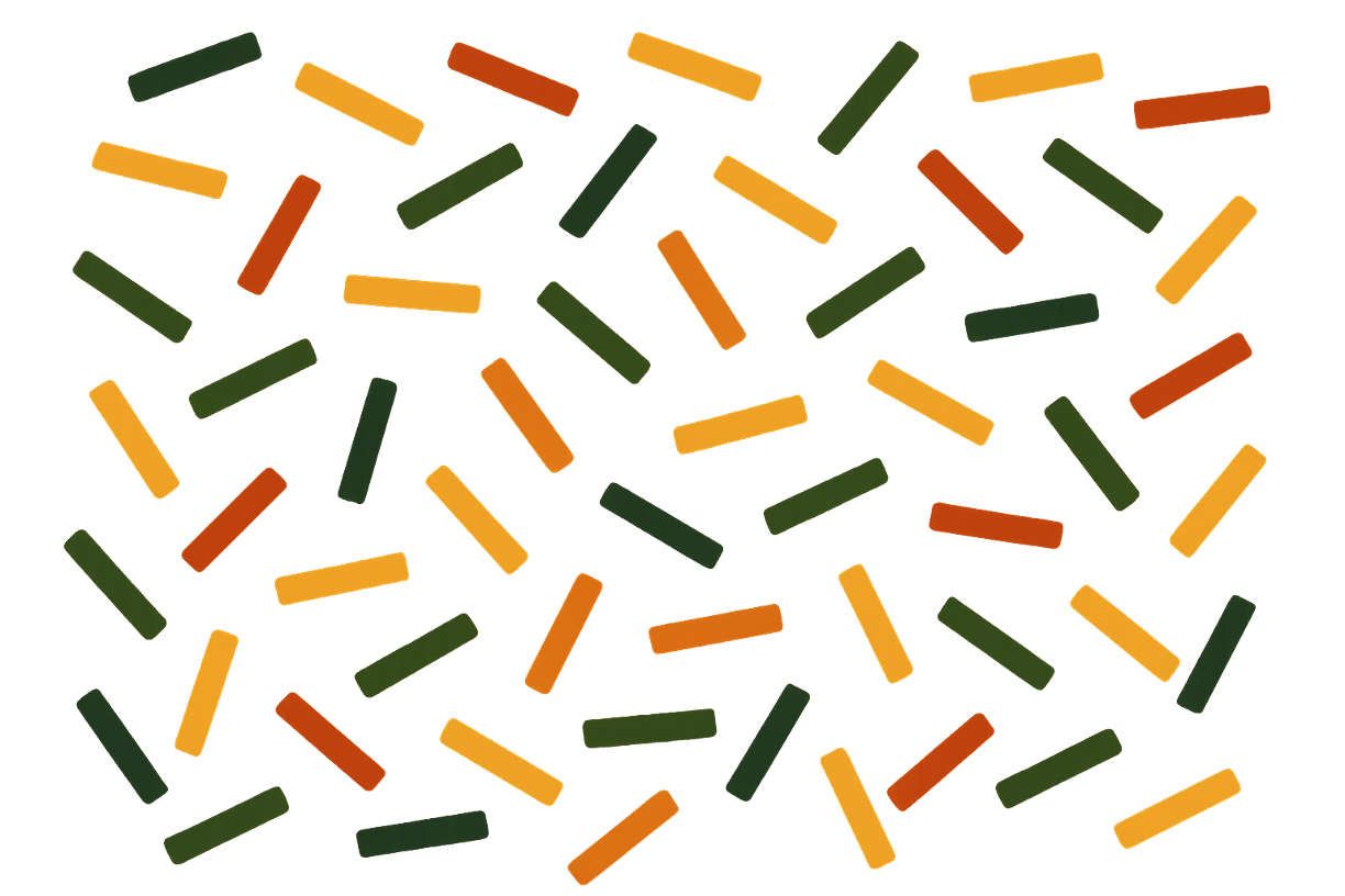
Side note: Types of RNA
From BioRender
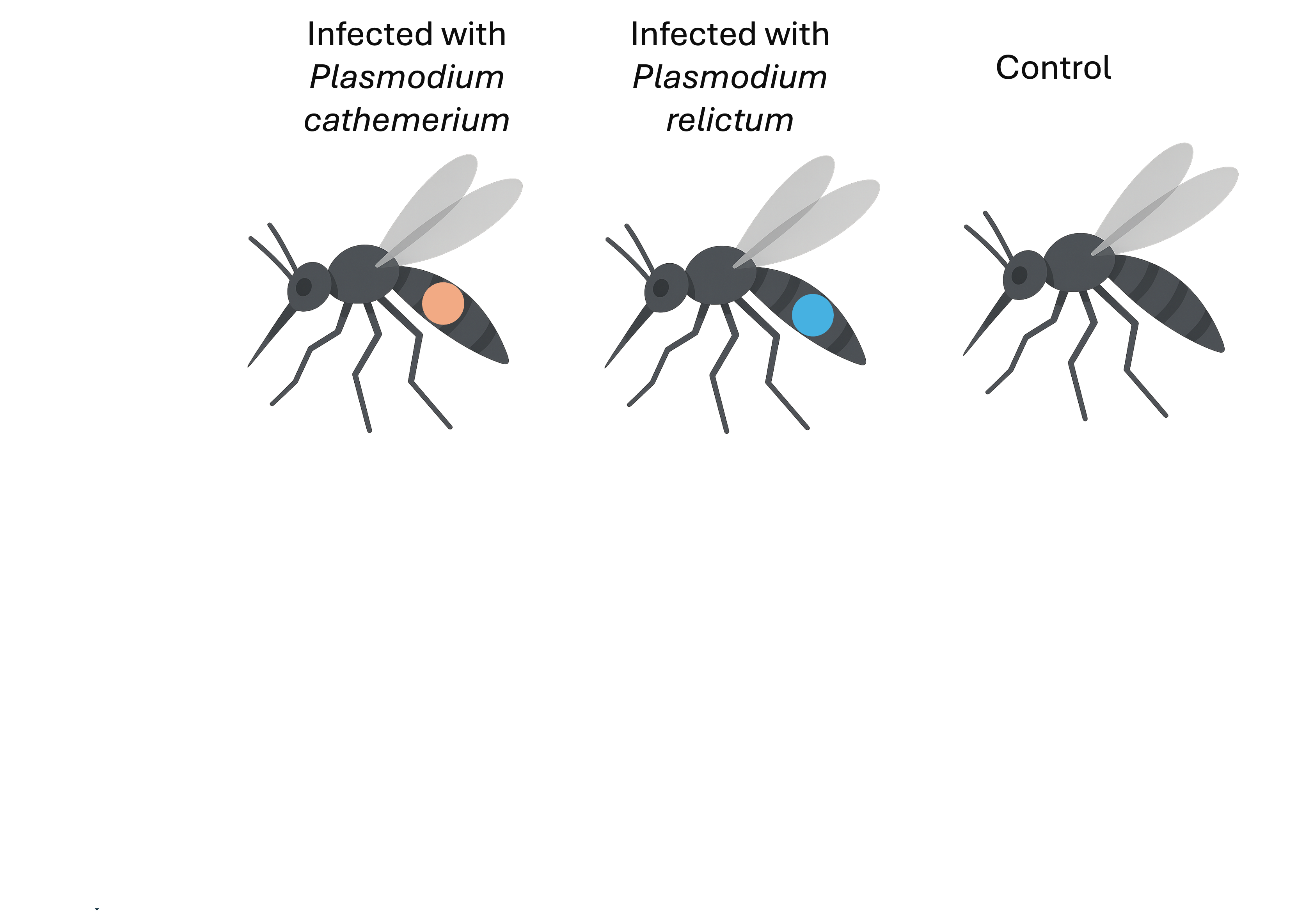
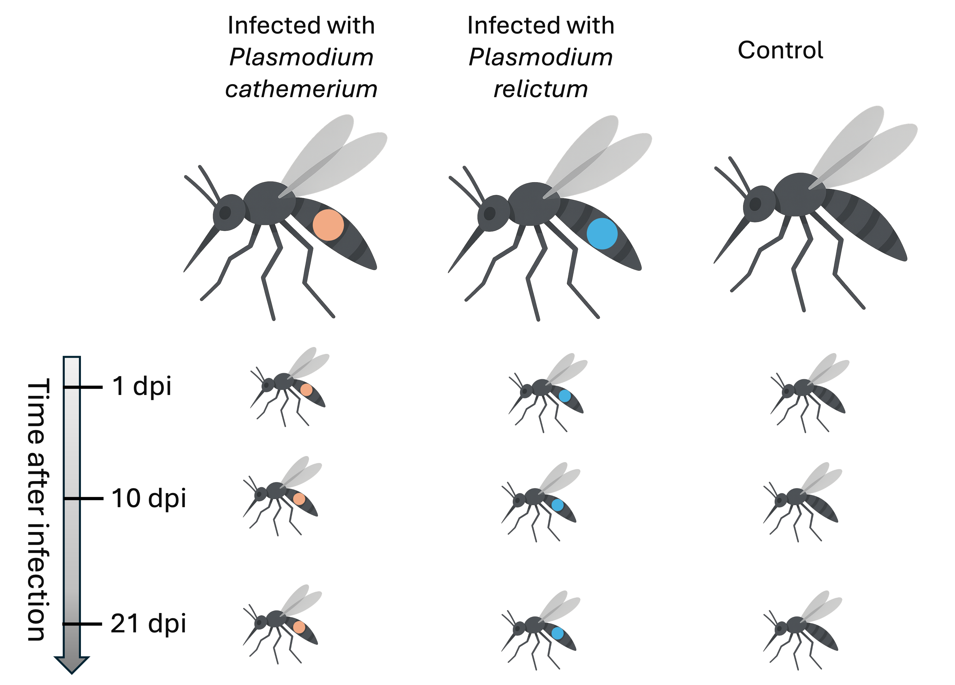
The Garrigós et al. experimental design
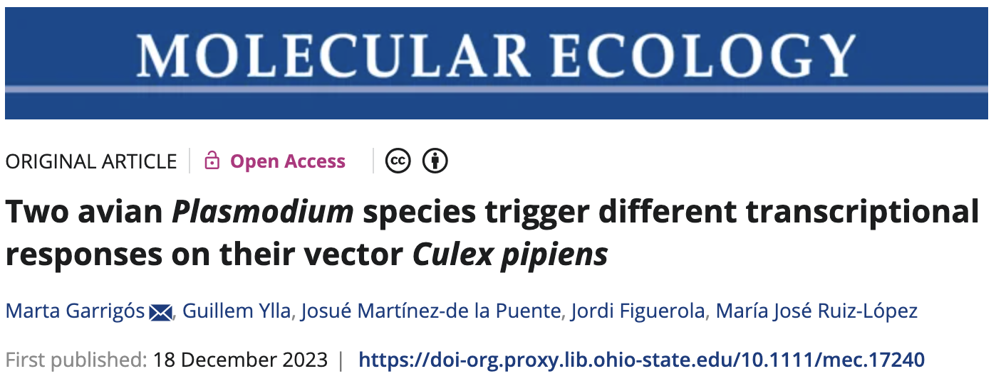
Garrigós et al. (2025)
Culex pipiens mosquitos infected with malaria-causing Plasmodium protozoans:
- Plasmodium relictum – higher virulence, lower tranmission rate
- Plasmodium cathemerium – lower virulence, higher tranmission rate
The Garrigós et al. experimental design
The Garrigós et al. experimental design
The Garrigós et al. experimental design
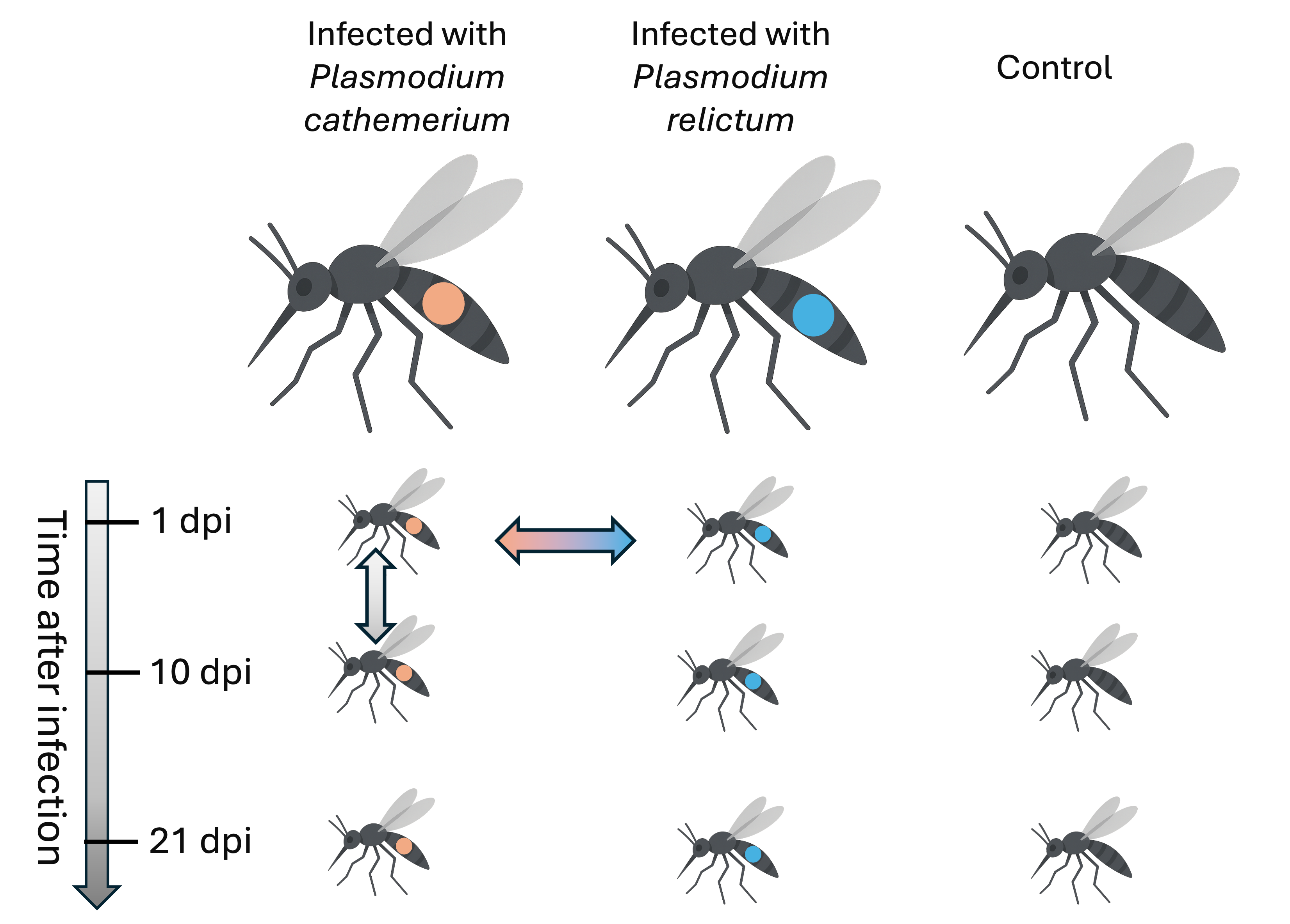
Experimental design
With this experimental design, would it be appropriate to sequence 9 samples total?
No – see the next slide
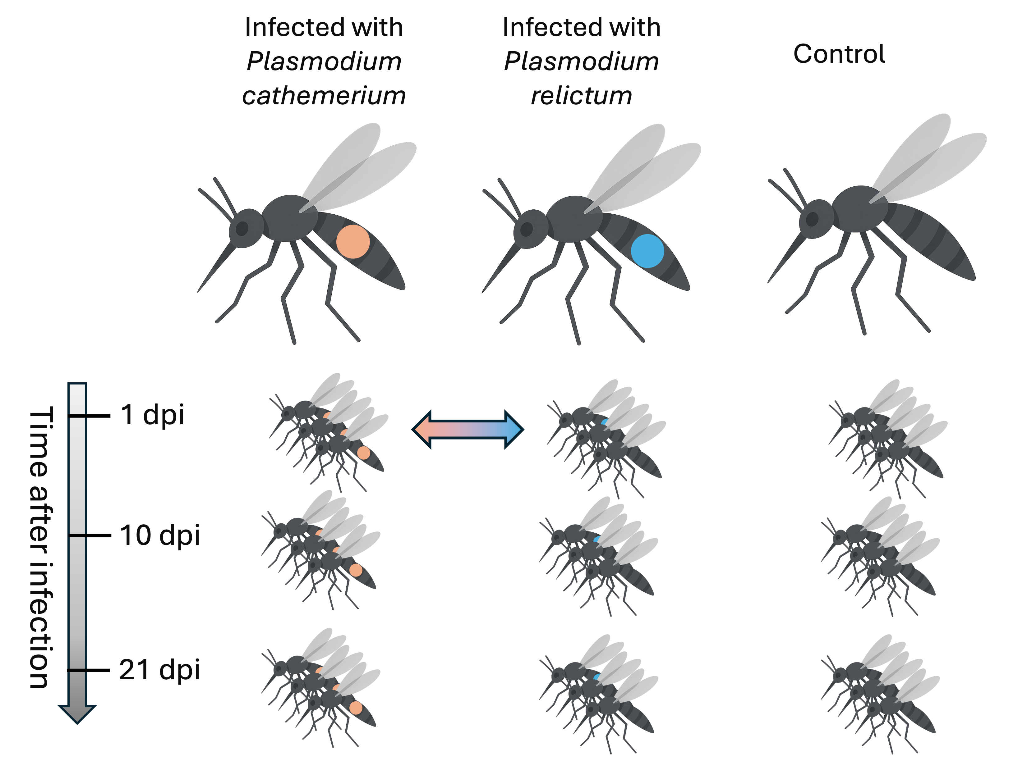
Experimental design: Biological replicates
To make statistically supported conclusions about expression differences,
we need biological replication (at least 3-5 samples per group):
From samples to reads
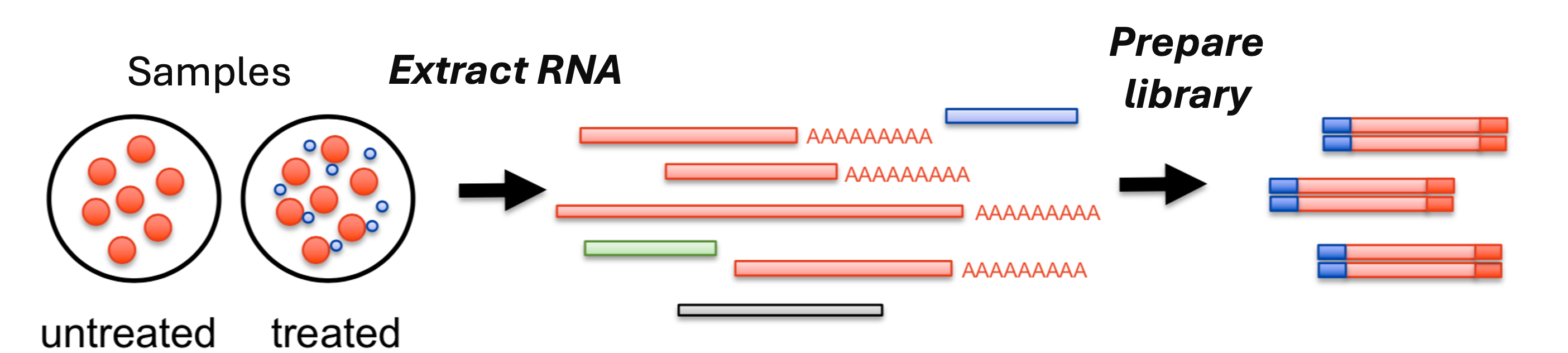
Which type of RNA do the red bars followed by AAAAAAA represent?
These are the mRNAs, which have poly-A tails (AAAAAA...)
From samples to reads
We want mRNAs but these often make up only a few percent of RNAs!
The two main ways to select for mRNAs are poly-A selection and ribo-depletion.
As mentioned in the previous lecture:
Library preparation is typically done by sequencing facilities / companies
Many samples can be “multiplexed” into a single (RNA-Seq) library
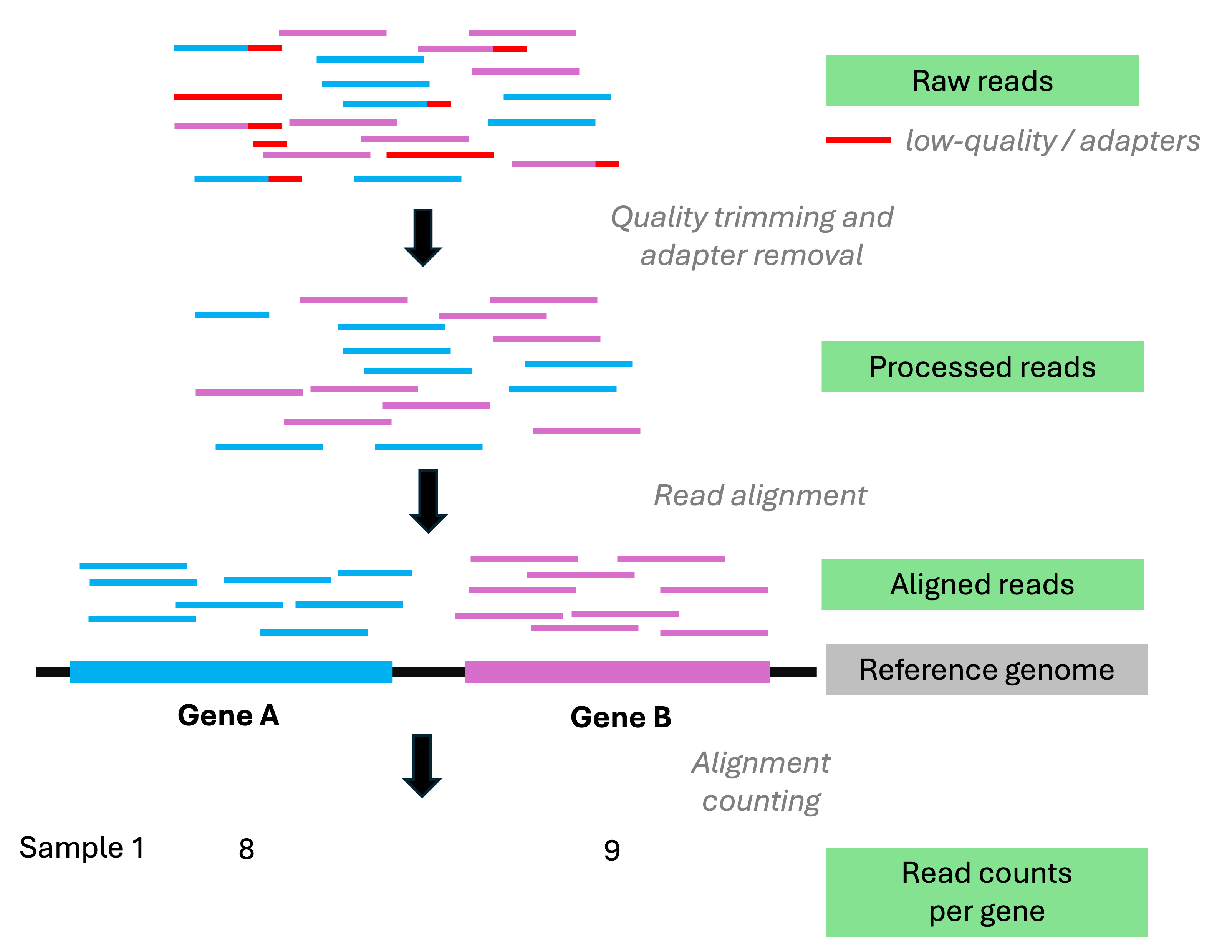
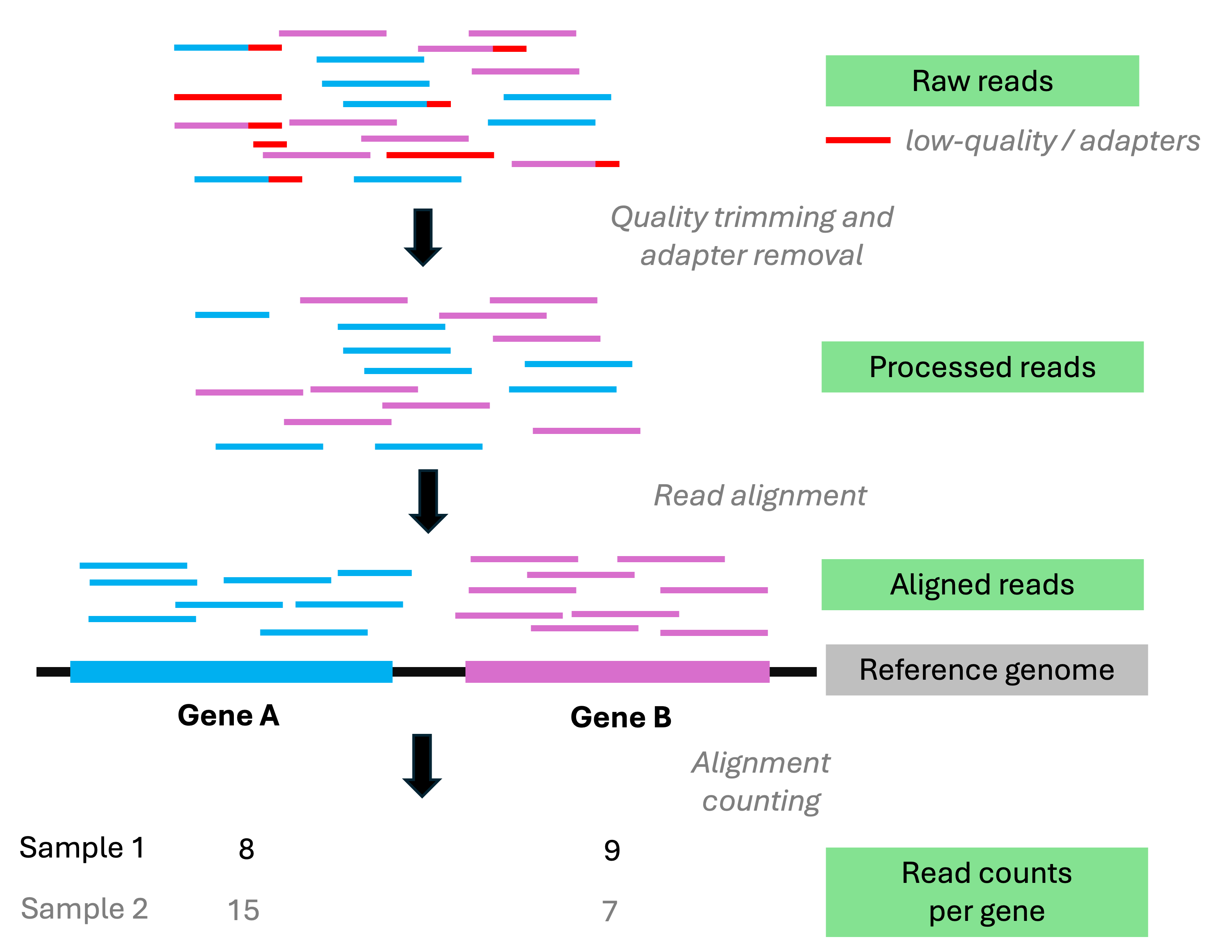
From samples to reads
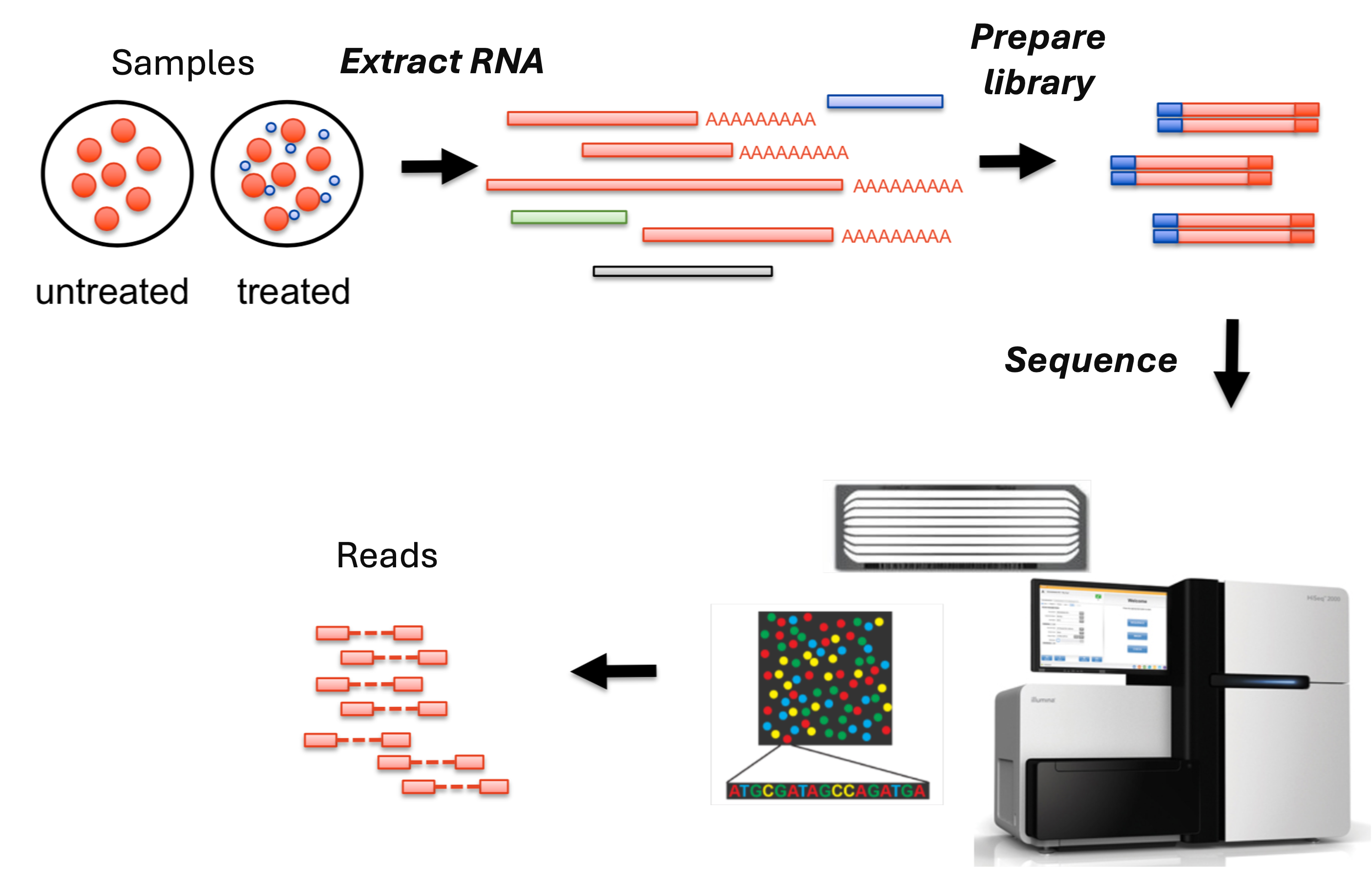
Modified after https://sydney-informatics-hub.github.io
A genAI diagram that explains RNA-Seq analysis
I though I’d get some generative AI help with the diagram on the previous slide –
this is what Adobe Firefly came up with: 😵💫
Side note: Splicing
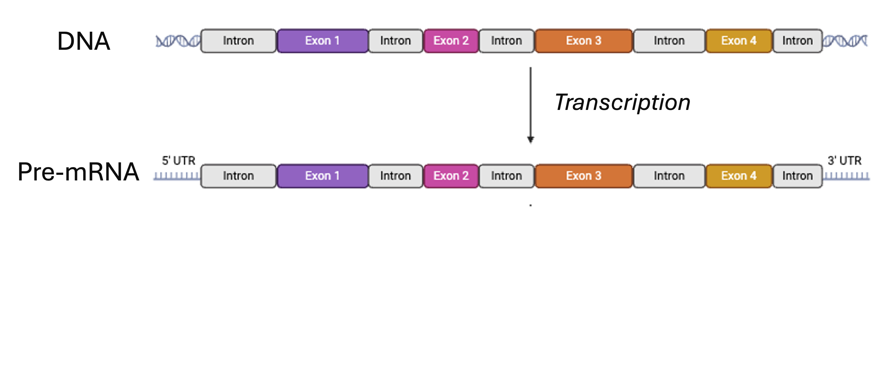
From BioRender
Side note: Splicing
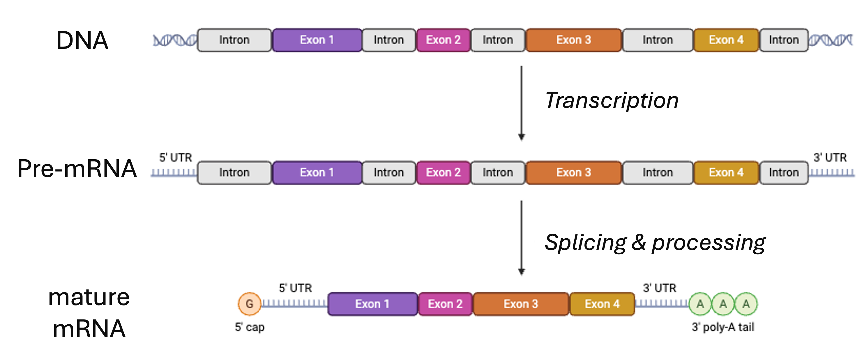
From BioRender
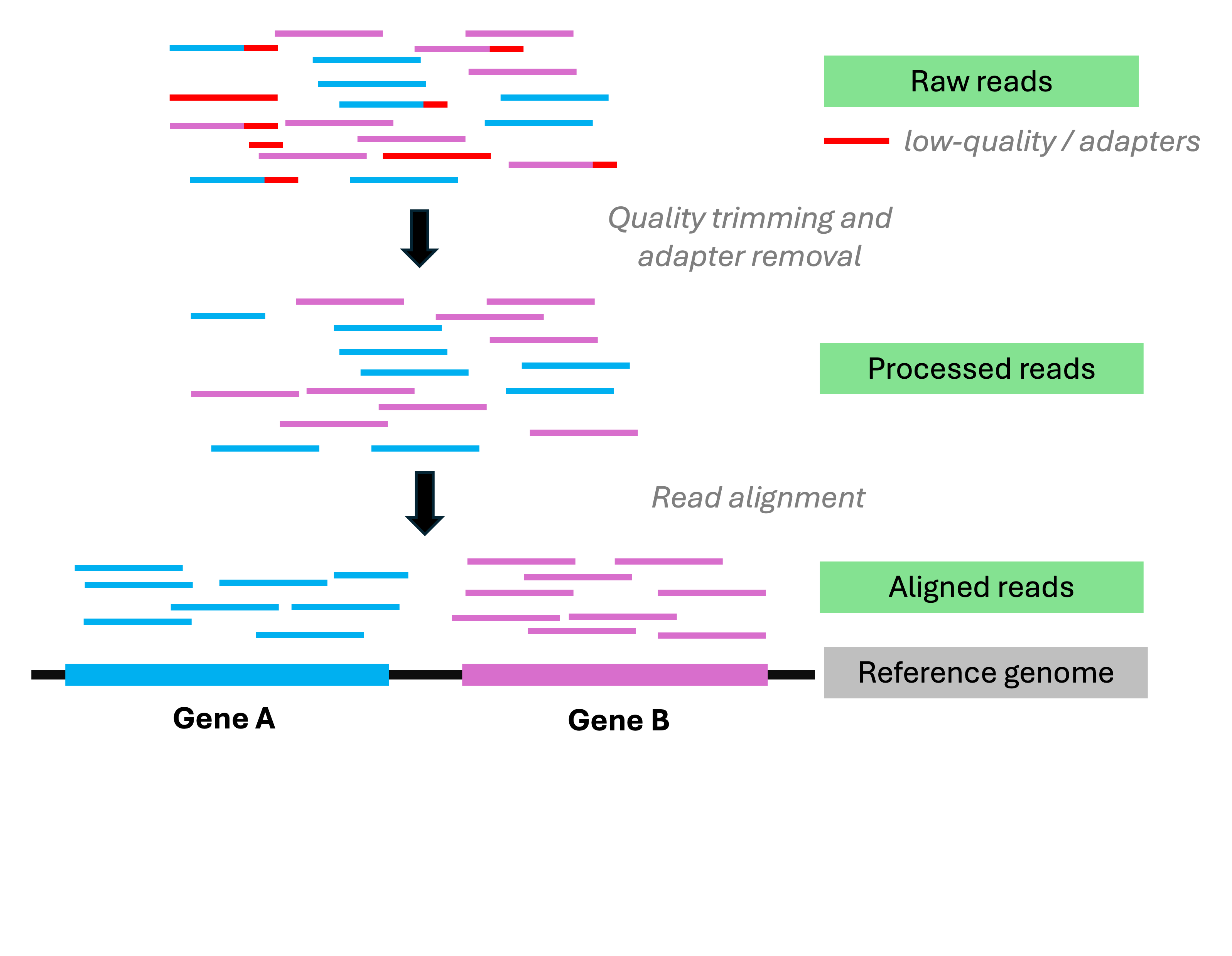
Read alignment to a reference genome
So, the alignment of reads to a reference genome needs to be “splice-aware”:
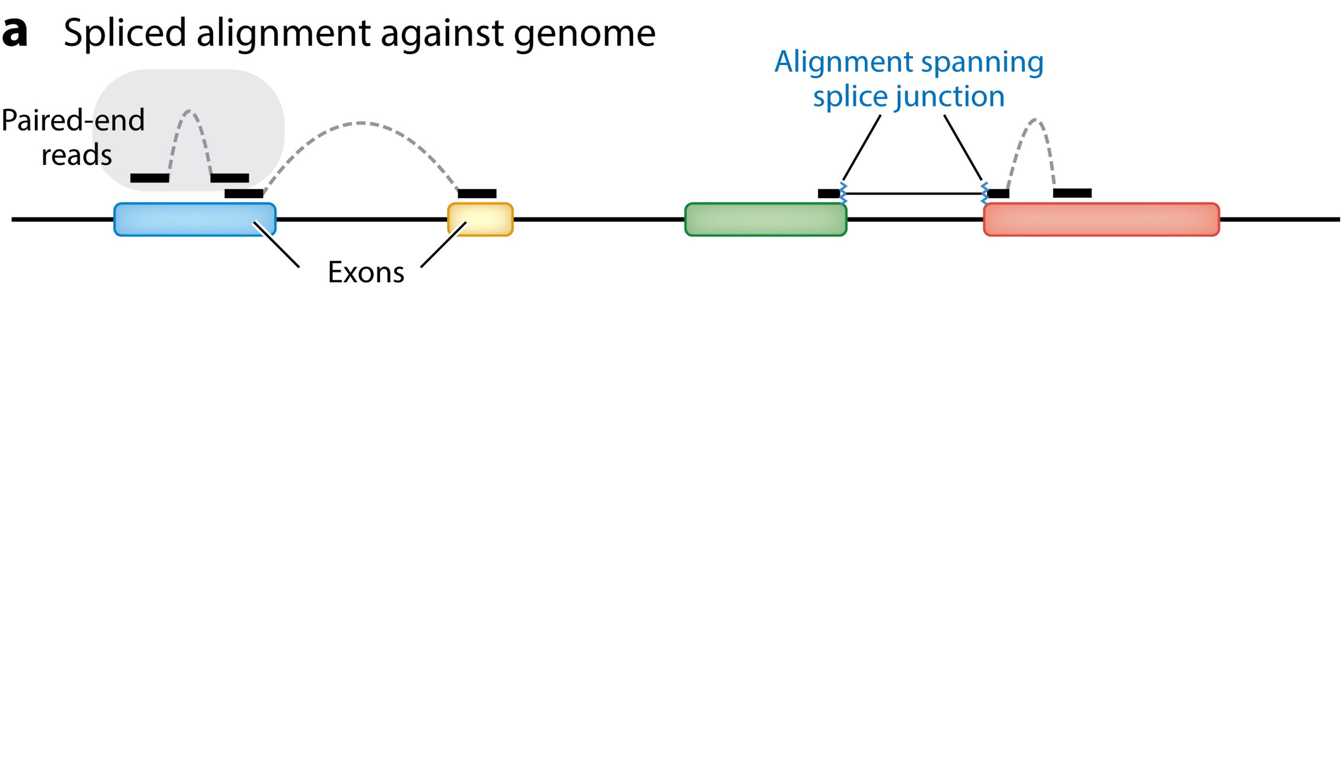
Van den Berge et al. (2019)
Read alignment to a reference genome
Alternatively, you can align to the transcriptome (i.e., all mature transcripts):
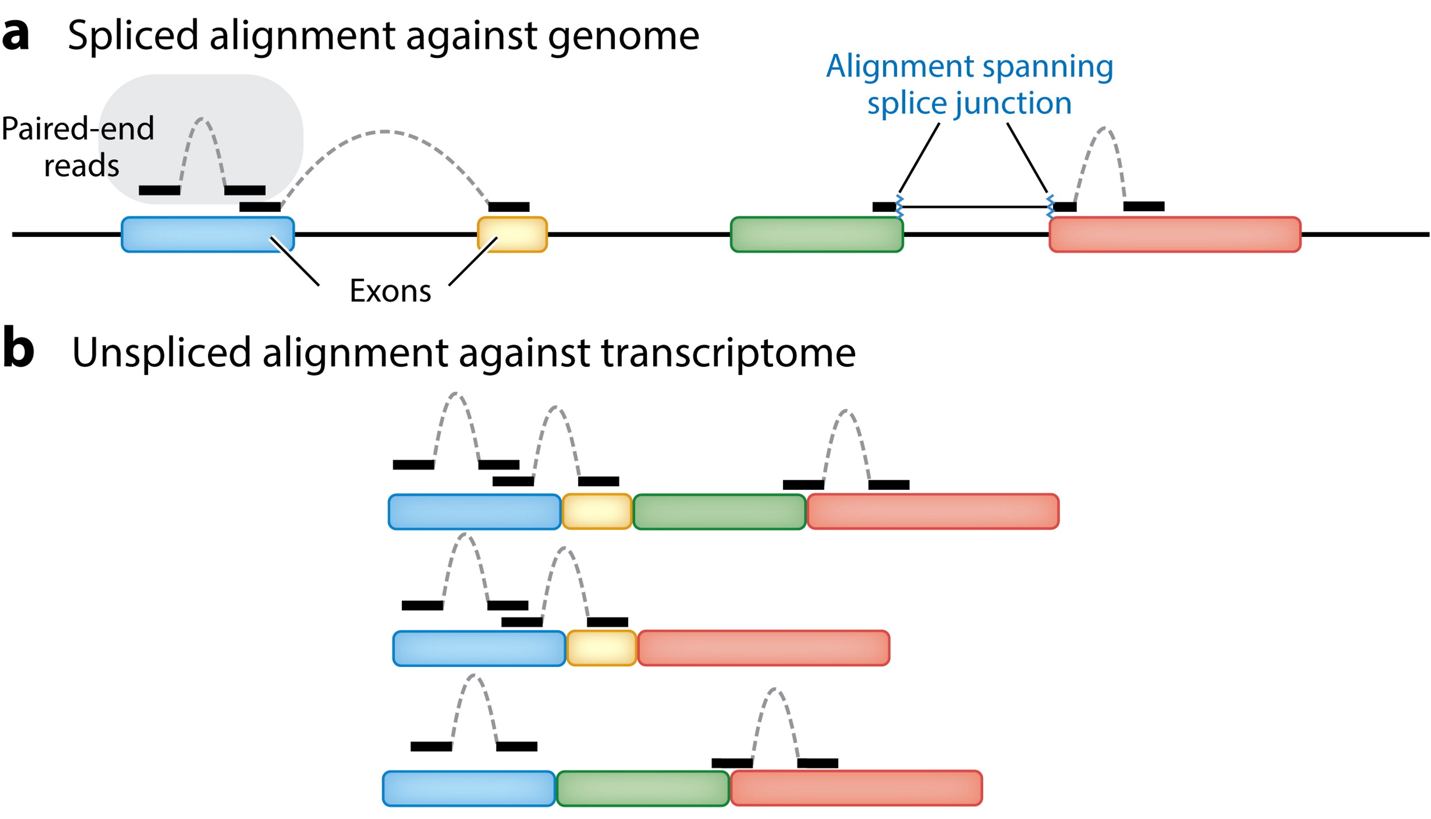
Van den Berge et al. (2019)
Read alignment to a reference genome
Why are there multiple bars in panel b? What do these represent?
These represent different transcripts originating from the same gene due to alternative splicing. These will produce different proteins, which are called isoforms.
Most short-read RNA-Seq studies do not attempt to distinguish between isoforms,
but rather quantify expression at the gene level.
Van den Berge et al. (2019)
Gene-wise quantification
In essence, a simple counting exercise once you have the alignments in hand:
for each sample, how many reads map to each gene?
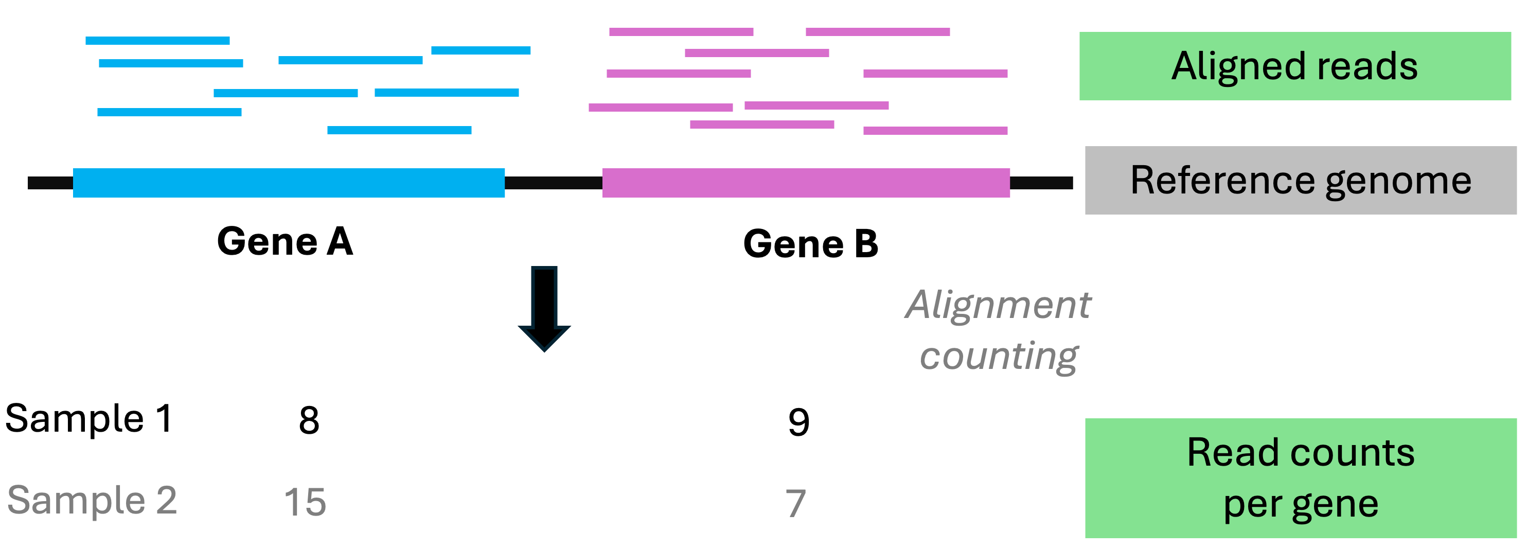
Though in practice, a bit more complicated than this, due to e.g.:
- Reads that map to multiple genes (“multi-mapping reads”)
- Sequencing biases and RNA fragmentation
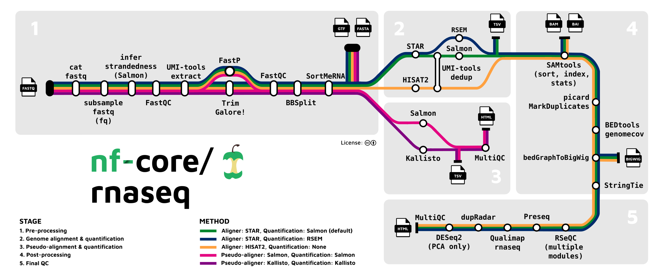
A best-practice pipeline to produce counts
The “nf-core” initiative (https://nf-co.re, Ewels et al. (2020)) aims to produce best-practice and automated bioinformatics pipelines, like for RNA-Seq (https://nf-co.re/rnaseq):
Principal Component Analysis (PCA)
PCA examines overall patterns of dissimilarity among samples,
such as whether groups of interest form distinct clusters:
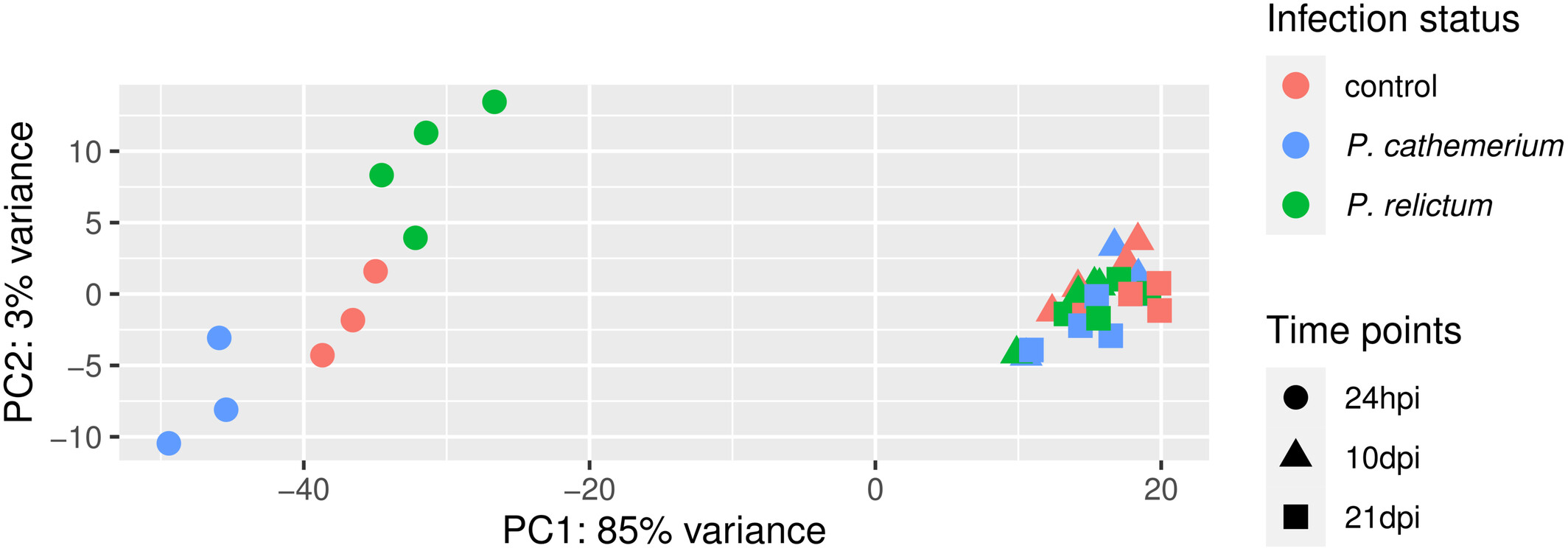
Fig. 1 from Garrigós et al. (2025)
We’ll talk more about the interpretation of this PCA plot in tomorrow’s lab
Principal Component Analysis (PCA)
PCA examines overall patterns of dissimilarity among samples,
such as whether groups of interest form distinct clusters:
Fig. 1 from Garrigós et al. (2025)
PCA is a very useful technique, not just for RNA-Seq data.
To learn more about how it works, see this video (short overview) and this video (more detailed).
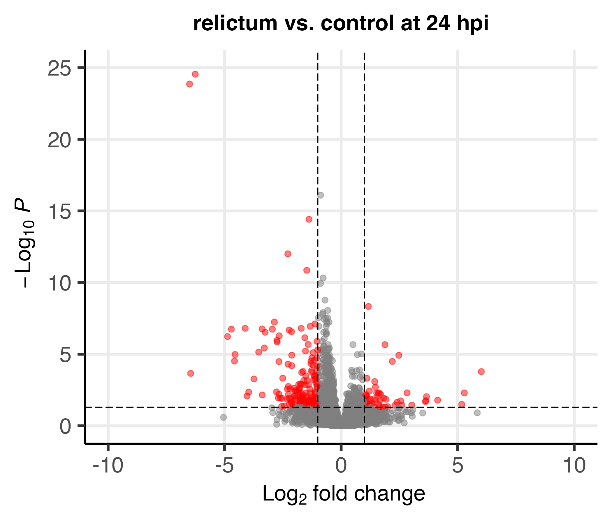
Differential expression (DE) analysis
Differential Expression (DE) analysis allows you to test, separately for every expressed gene in your dataset, whether it significantly differs in expression level between groups.
Typically, this is done with pairwise comparisons between groups:
Differential expression (DE) analysis
Differential Expression (DE) analysis allows you to test, separately for every expressed gene in your dataset, whether it significantly differs in expression level between groups.
Typically, this is done with pairwise comparisons between groups:
Functional enrichment: GO
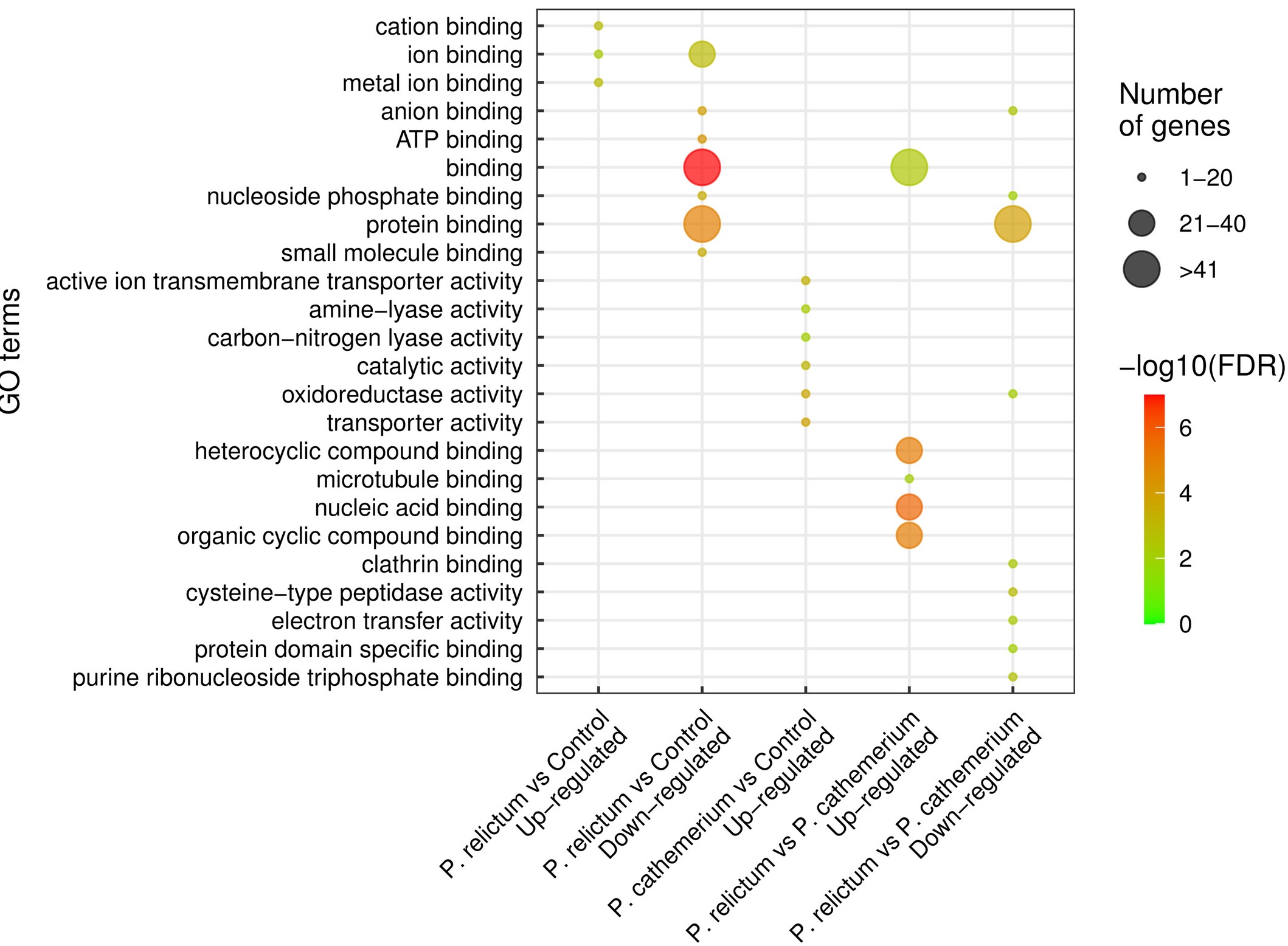
Fig. 4 from Garrigós et al. (2025)
Functional enrichment: KEGG

Rodriguez et al. (2020)
KEGG representation of up-regulated genes related to jasmonic acid (JA) signal transduction pathways (ko04075) in banana cv. Calcutta 4 after inoculation with Pseudocercospora fijiensis. Genes or chemicals up-regulated at any time point were highlighted in green.
