Week 3 lab — part 1:
Computational Infrastructure
1 Introduction to the lab
In today’s lab:
We will start with learning about a typical “computational infrastructure” to analyze high-throughput sequencing (HTS) data — this page.
We will then use that infrastructure to start the exploration of an HTS dataset. We’ll check out reference genome and HTS read files, and perform read quality control – the next page.
2 Computational infrastructure overview
Due in large part to the amount of data involved, a laptop or desktop computer is often not sufficient to work with HTS data, or with large-scale genomics and transcriptomics data more generally.
Additionally, most of the specialized programs that help you analyze your data can only be run through a “command-line interface”.
Therefore, a typical computational infrastructure to do what we may call “command-line genomics” involves:
- A supercomputer1 — in our case, the Ohio Supercomputer Center (OSC)
- A text editor — I recommend and will demonstrate VS Code
- The Unix shell (terminal)
- R (or perhaps Python) for interactive statistical analysis and visualization.
Today, we will go through the first three of the abovementioned items: on this page, we’ll get familiar with them, and on the next page, we’ll apply what we learned to some reference genome and HTS read data.
In the lab next week, we will cover the fourth in the context of RNA-seq differential expression analysis.
If you will often be doing genomics projects like the ones mentioned above, it’s hard to avoid using this (kind of) infrastructure. But here are some conditions in which you might reasonably avoid it:
- You’re doing a single genomics project, your main research focus is elsewhere
- You’re willing to outsource part of the analysis
Note that for several types of HTS projects, including those involving metabarcoding or RNA-seq data (as we’ll see next week), the analysis consists of two distinct parts:
- The first is compute-heavy and involves command-line programs; it is also quite standardized, and therefore suitable to be outsourced.
- The second can be done on a laptop and in terms of coding only requires R
You could also try a platform like Galaxy, which has a web browser interface and doesn’t require coding — but I wouldn’t recommend this if you’re going to do multiple genomics projects.
Advantages of Command-Line Interfaces (CLIs) over “Graphical User Interfaces” (GUIs) include:
Efficiency — A CLI allows you to write a simple loop to run it in the same way for many samples.
(In combination with usage of a supercomputer, you can process all those samples in parallel.)Reproducibility — You can easily save all commands & scripts, making it straightforward to rerun/adapt an analysis.
3 The Ohio Supercomputer Center (OSC)
3.1 Introduction to supercomputers
A supercomputer is a highly interconnected set of many computer processors and storage units. You can think of it simply as a network of computers — with individual computers called “nodes”.
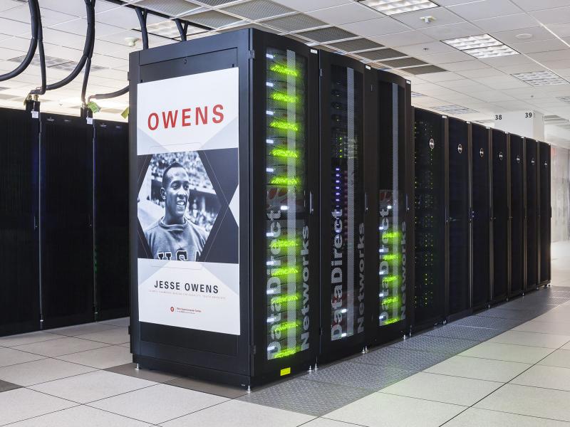
Supercomputers are also commonly referred to as High-Performance Computing (HPC) clusters or simply compute clusters. This is what Owens, one of the OSC supercomputers, physically looks like:
Why you might need a supercomputer:
- Often, your genomics dataset is too large to be handled efficiently, or at all, by a laptop/desktop computer.
- To speed up long-running analyses by using more computing power, and repeated analyses (like the independent alignment of reads for different samples) by running them in parallel.
- It’s also a great place to store large amounts of data — and genomics data is often very large.
3.2 Introduction to OSC

The Ohio Supercomputer Center (OSC) provides computing resources to researchers (and others) across Ohio. OSC has two supercomputers/clusters (named Owens and Pitzer), and lots of infrastructure for their usage. Research usage is charged at subsidized rates, and in most case, these costs are absorbed at the college level.
The structure of an OSC supercomputer
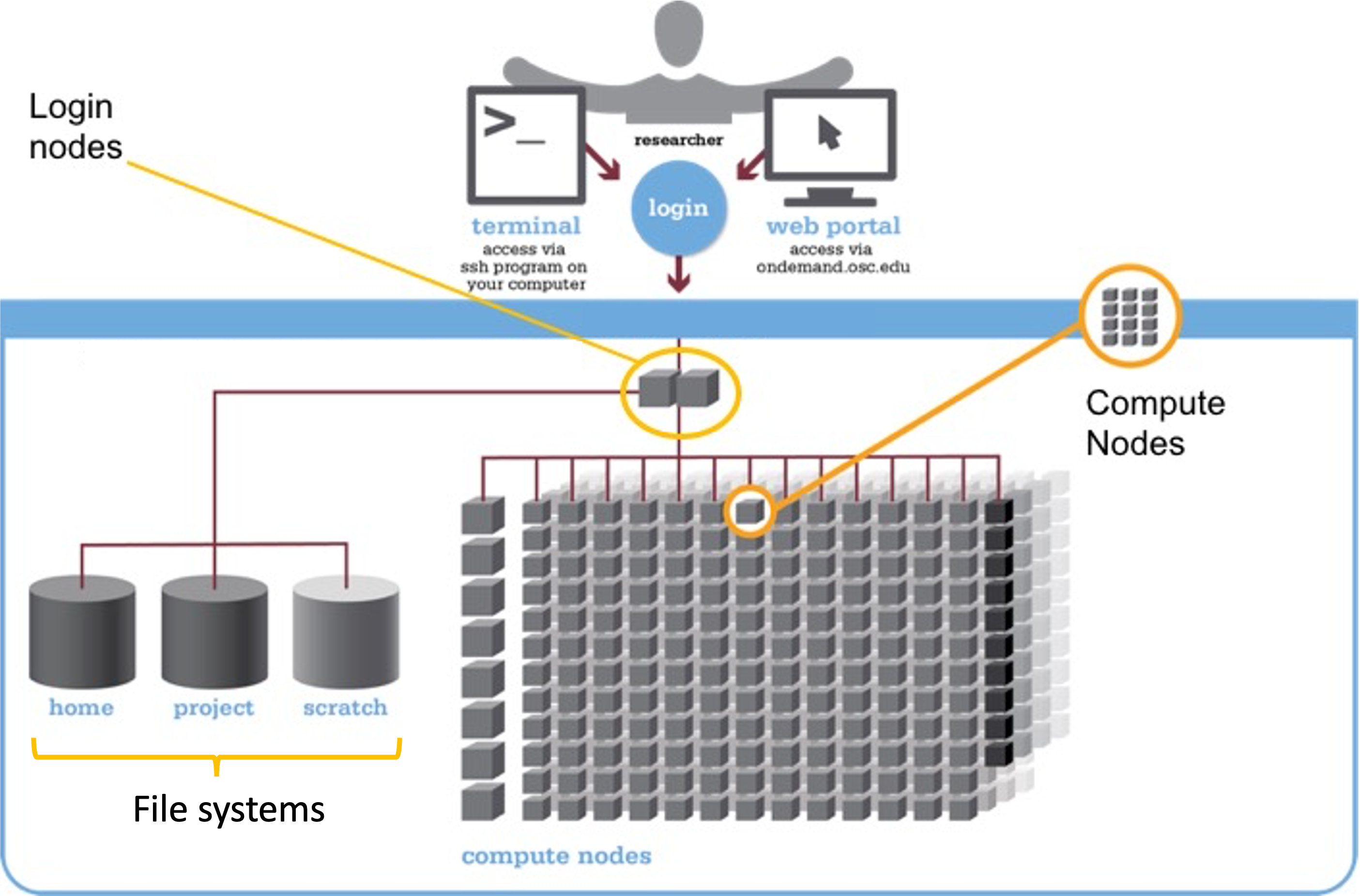
We can think of a supercomputer as having three main parts:
- File Systems: Where files are stored (these are shared between the two OSC clusters)
- Login Nodes: The handful of computers everyone shares after logging in
- Compute Nodes: The many computers you can reserve to run your analyses
Compared to command-line computing on a laptop or desktop, the following aspects are different when working on a supercomputer like at OSC:
- Login versus compute nodes
“Login nodes”, the nodes you end up on after logging in, are not meant for heavy computing and you have to request access to “compute nodes” to run most analyses. - “Non-interactive” computing is common
It is common to write and “submit” scripts to a queue instead of running programs interactively. - Software
You generally can’t install “the regular way”, and a lot of installed software needs to be “loaded” (as we’ll see today). - Operating system
Supercomputers run on the Linux operating system
3.3 The OSC OnDemand web portal
Go to https://ondemand.osc.edu and log in with your OSC (not OSU!) credentials.
You should see a landing page similar to the one below:
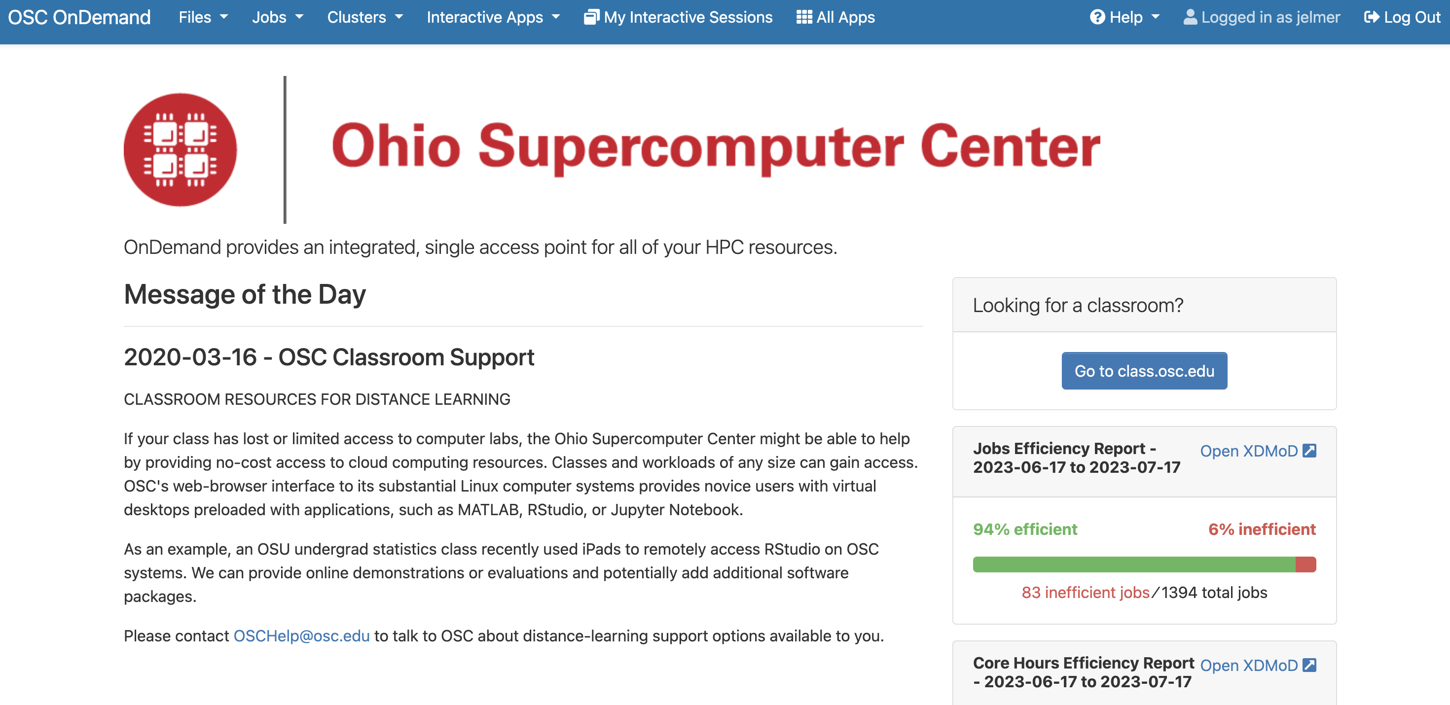
We will now go through some of the dropdown menus in the blue bar along the top.
Files: File system access
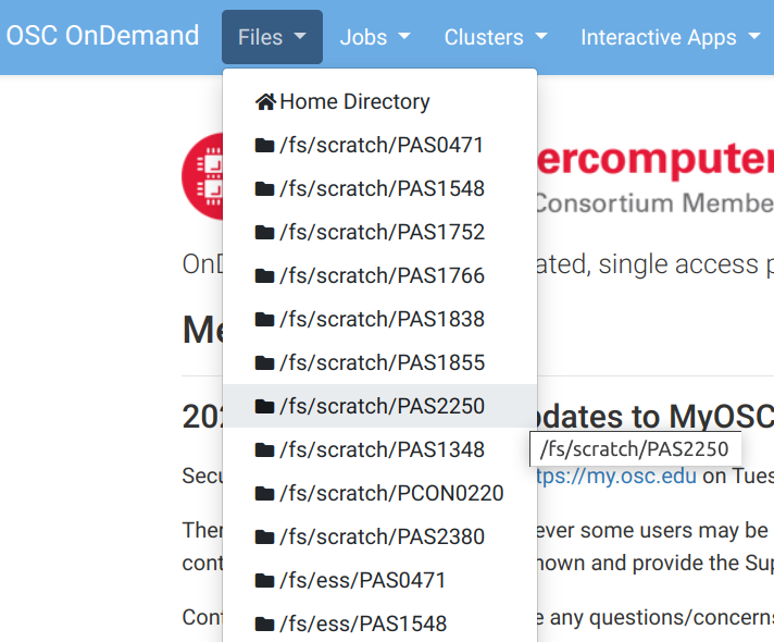
Hovering over the Files dropdown menu gives a list of directories (=folders, and “dir” for short) that you have access to. If your account is brand new, you should only two directories listed2:
- A Home directory (starts with
/users/) - A project “scratch” directory (starts with
/fs/scratch/)PAS2250
Select the PAS2250 scratch directory, /fs/scratch/PAS2250, where we’ll be working today and next week:
Once there, you should see a list of directories and files (here: just a single dir), and you can click on the directories to explore the contents further:
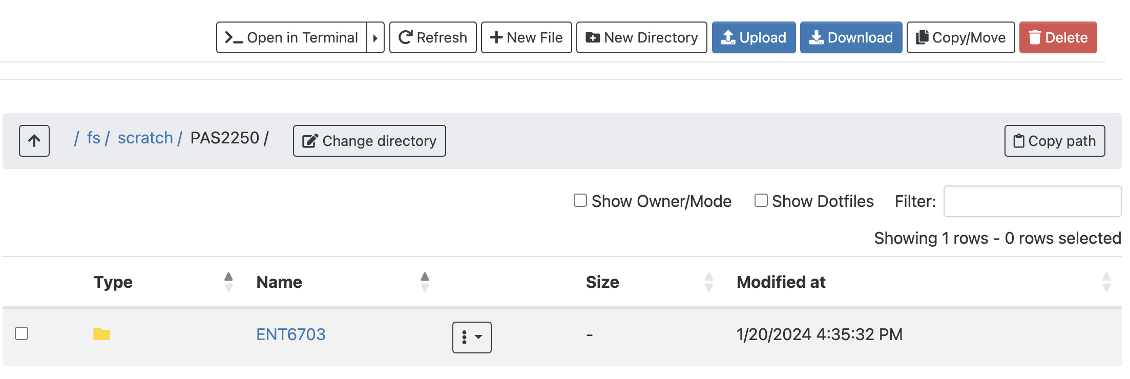
This interface is much like the file browser on your own computer, so you can also create, delete, move and copy files and folders, and even upload (from your computer to OSC) and download (from OSC your computer) files3 — see the buttons across the top.
Your Turn: Create your own folder (click to see instructions)
- Click your way into
ENT6703within/fs/scratch/PAS2250if you’re not already there. - You should (at least) see directories/folders named
shareandjelmer. - Create your own folder by clicking the
New Directorybutton at the top. - Please give it the exact same name as your OSC username (including any capitalization).
(You can see what your username is by looking at the right side of the blue top bar:)

Clusters: Unix shell access
Interacting with a supercomputer is most commonly done using a Unix shell, and we’ll learn about the basics of doing so soon. Under the Clusters dropdown menu, you can access a Unix shell either on Owens or Pitzer:
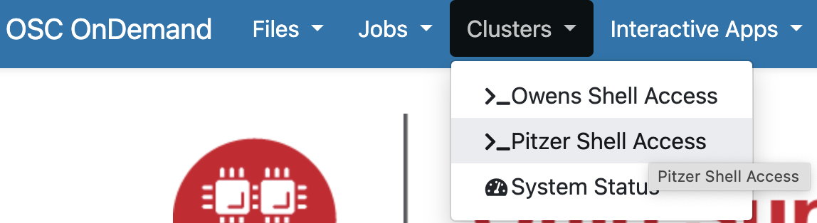
I’m selecting a shell on the Pitzer supercomputer, which will open a new browser tab looking like this:
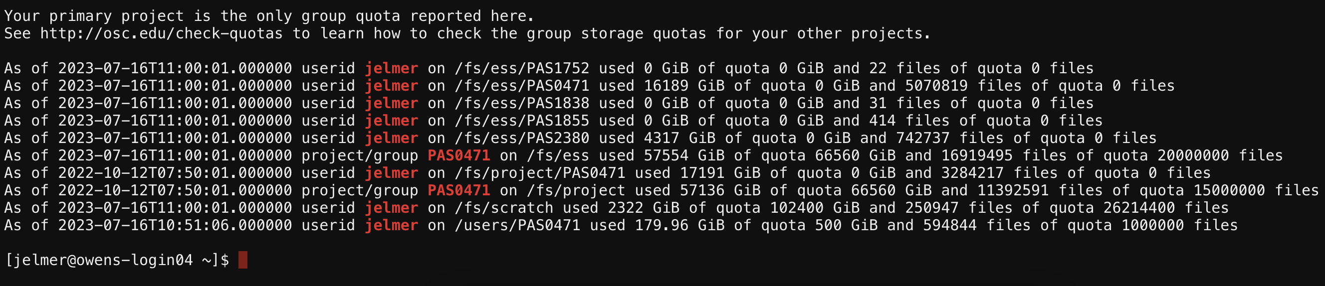
However, from now on, we’ll be accessing a Unix shell inside the VS Code text editor, which also gives us some additional functionality in a user-friendly way.
Interactive Apps
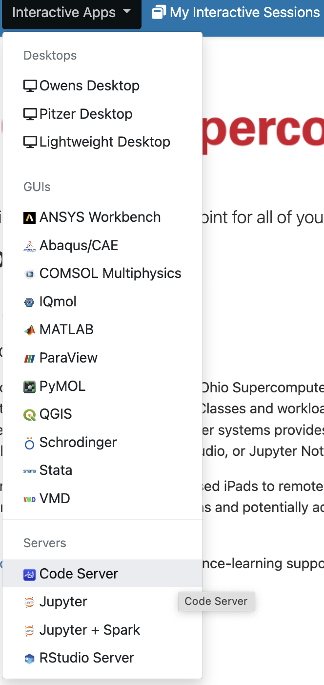
We can access programs with Graphical User Interfaces (GUIs; point-and-click interfaces) via the Interactive Apps dropdown menu — let’s select VS Code using the “Code Server” button:
4 The VS Code text editor
4.1 What is VS Code?
VS Code (in full, Visual Studio Code) is basically a fancy text editor.
To emphasize the additional functionality relative to basic text editors like Notepad and TextEdit, editors like VS Code are also referred to as “IDEs”: Integrated Development Environments. The RStudio program is another good example of an IDE. For our purposes:
- VS code will be our IDE for Unix shell code (this week)
- RStudio will be our IDE for R (in the differential expression lab next week)
4.2 Connecting to VS Code
Because Interactive Apps like VS Code and RStudio run on compute nodes (not login nodes), which need to be “reserved”, we have to fill out a form and specify the following details (see also the screenshot below):
| Option | Value |
|---|---|
The OSC Project that should be billed for the compute resource usage |
PAS2250 |
The Number of hours we want to make a reservation for4 |
4 |
The Working Directory5 for the program |
your newly-created personal folder in /fs/scratch/PAS2250/ENT6703 (e.g. /fs/scratch/PAS2250/ENT6703/jelmer) |
The Codeserver Version |
4.8 |
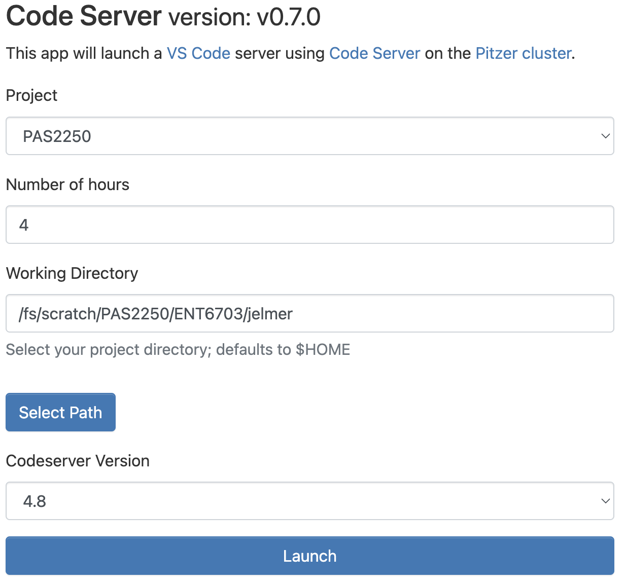
Click on Launch at the bottom, which will send your request to the “compute job” scheduler. First, your job will be “Queued” — that is, waiting for the job scheduler to allocate resources on the compute nodes to it:
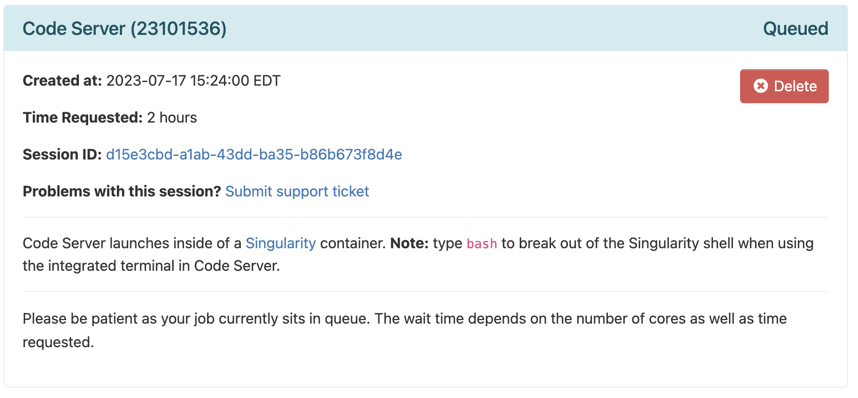
Your job is typically granted resources within a few seconds (the card will then say “Starting”), and be ready for usage (“Running”) in another couple of seconds:
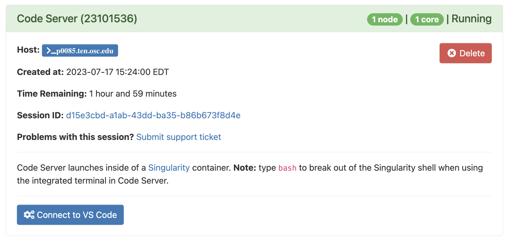
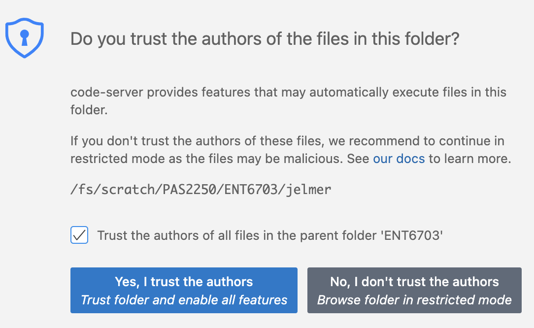
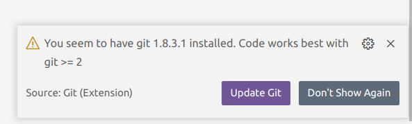
Then, click on the blue Connect to VS Code button to open VS Code in a new browser tab. When VS Code opens, you may get these two pop-ups — click “Yes” (and check the box) and “Don’t Show Again”, respectively:
4.3 The VS Code User Interface
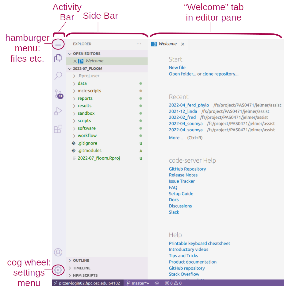
Side bars
The Activity Bar (narrow side bar) on the far left has:
- A (“hamburger menu”), which has menu items like
Filethat you often find in a top bar. - A (cog wheel icon) in the bottom, through which you can mainly access settings.
- Icons to toggle (wide) Side Bar options — but we’ll only use the default selection, the Explorer (file browser)
Editor pane and Welcome document
The main part of the VS Code is the editor pane. Here, we can open files like scripts and other types of text files, and images. (Whenever you open VS Code, an editor tab with a Welcome document is automatically opened. This provides some help and some shortcuts like to recently opened files and folders.)
Terminal (with a Unix shell)
Open a terminal by clicking => Terminal => New Terminal.
Your Turn: Try a few color themes (click to see instructions)
- Access the “Color Themes” option by clicking =>
Color Theme. - Try out a few themes and see what you like!
5 The Unix shell
5.1 What is the Unix shell?
A computer’s shell is an interface inside a Terminal window that allows you to interact with your computer by typing commands. It is also referred to as the the “command line” — with “command-line tools/programs” being software that is run using shell commands.
The Unix shell is the shell of Unix-based operating systems, which include Mac and Linux (but not Windows).
We’ll now learn a couple of Unix shell commands, to familiarize yourself with working in this environment.
Doing so is also useful because in many ways, you can think of using a command-line bioinformatics program as using just another Unix command. Therefore, our skills with Unix commands will extend to using command-line bioinformatics tools!
5.2 First steps in the Unix shell
The prompt
Inside your terminal, the “prompt” indicates that the shell is ready for a command. Your prompt at OSC should show the following pieces of information:
[<username>@<node-name> <working-dir>]$For example:
[jelmer@p0080 jelmer]$ You type your command line expressions after the dollar sign $, and then press Enter to execute them. When it has finished executing, we’ll get our prompt back and can type a new command.
The gray boxes like the ones shown above will be used to show the command line expressions that you should type.
In upcoming boxes, the prompt itself (
[...]$) will not be shown, but only the command line expressions that you type. This is to save space and to allow you for copy-and-pasting (but I recommend typing!).Paler gray boxes (below the boxes with command have & with italic text) show the output of commands.
A few simple commands: date, whoami, pwd
The Unix shell comes with hundreds of “commands”: small programs that perform specific actions. If you’re familiar with R or Python, a Unix command is like an R/Python function.
Let’s start with a few simple commands:
- The
datecommand prints the current date and time:
dateFri Jan 26 14:31:51 EST 2024- The
whoami(who-am-i) command prints your username:
whoamijelmer- The
pwd(Print Working Directory) command prints the path to the directory you are currently located in:
pwd/fs/scratch/PAS2250/ENT6703/jelmerAll 3 of those commands provided us with some output. That output was printed to screen, which is the default behavior for nearly every Unix command.
When working in a Unix shell, you are always “in” a specific directory and this is called your working directory.
In a path (= location of a file or directory) such as that output by
pwd, directories are separated by forward slashes/. (And a leading forward slash, if present, indicates the computer’s root directory.)
Everything in the shell is case-sensitive, including commands and file names.
Avoid spaces in file and directory names! Use e.g. underscores or capitalization to distinguish words.
5.3 cd and command actions & arguments
In the above three command line expressions:
- We merely typed a command and nothing else
- The command provided some information, which was printed to screen
But many commands perform an action other than providing information. For example, you can use the command cd to Change Directory (i.e. change your working dir). And like many commands that perform an action, cd normally has no output at all.
Let’s use cd to move to another directory by specifying the path to that directory after the cd command:
cd /fs/scratch/PAS2250/ENT6703/sharepwd/fs/scratch/PAS2250/ENT6703/shareIn more abstract terms, what we did above was to provide cd with an argument, namely the path of the dir to move to. Arguments generally tell commands what file or directory to operate on.
As we’ve seen, then, cd gives no output when it succesfully changed the working directory. But let’s also see what happens when it does not succeed — it gives an error:
cd /fs/Scratch/PAS2250bash: cd: /fs/Scratch/PAS2250: No such file or directoryYour Turn: What was the problem with the path we specified? (Click to see the answer)
We used a capital S in /Scratch/ — this should have been /scratch/.
As pointed out above, paths (dir and file specifications) are case-sensitive on Unix systems!
5.4 ls and command options
The default behavior of ls
The ls command, short for “list”, will list files and directories:
lsdata README.md(You should still be in /fs/scratch/PAS2250/ENT6703/share. If not, cd there first.)
ls output colors (click to expand)
Unfortunately, the ls output shown above does not show the different colors you should see in your shell — here are some of the most common ones:
- Entries in blue are directories (like
dataandmetadataabove) - Entries in black are regular files (like
README.mdabove) - Entries in red are compressed files (we’ll see an example soon).
This default way that ls shows the output can be changed by providing ls with options.
Options (to ls)
In general, whereas arguments tell a command what to operate on, options will modify its behavior. For example, we can call ls with the option -l (a dash followed by a lowercase L):
ls -l total 17
drwxr-xr-x 5 jelmer PAS0471 4096 Jan 21 12:39 data
-rw-r--r-- 1 jelmer PAS0471 1502 Jan 22 11:04 README.mdNotice that it lists the same items as our first ls call above, but printed in a different format: one item per line, with additional information included, such as the date and time each file was last modified, and the file sizes in bytes (to the left of the date).
Let’s add another option, -h:
ls -l -htotal 17K
drwxr-xr-x 5 jelmer PAS0471 4.0K Jan 21 12:39 data
-rw-r--r-- 1 jelmer PAS0471 1.5K Jan 22 11:04 README.mdYour Turn: What is different about the output, and what do you think that means? (Click to see the answer)
The only difference is in the format of the column reporting the sizes of the items listed.
We now have “Human-readable filesizes” (hence -h), where sizes on the scale of kilobytes will be shown with Ks, of megabytes with Ms, and of gigabytes with Gs. That can be really useful especially for very large files.
Conveniently, options can be pasted together as follows:
ls -lhCombining options and arguments
Arguments to ls should be dirs or files to operate on. For example, if we wanted to see what’s inside the data dir, instead of inside our working dir, we could type:
ls datafastq meta refThe data dir appears to contain three (sub)dirs with different kinds of data. We’ll talk in detail about that later, but for now let’s look inside the fastq dir:
ls data/fastqERR10802863_R1.fastq.gz ERR10802865_R2.fastq.gz ERR10802868_R1.fastq.gz ERR10802870_R2.fastq.gz ERR10802875_R1.fastq.gz ERR10802877_R2.fastq.gz ERR10802880_R1.fastq.gz ERR10802882_R2.fastq.gz ERR10802885_R1.fastq.gz
ERR10802863_R2.fastq.gz ERR10802866_R1.fastq.gz ERR10802868_R2.fastq.gz ERR10802871_R1.fastq.gz ERR10802875_R2.fastq.gz ERR10802878_R1.fastq.gz ERR10802880_R2.fastq.gz ERR10802883_R1.fastq.gz ERR10802885_R2.fastq.gz
ERR10802864_R1.fastq.gz ERR10802866_R2.fastq.gz ERR10802869_R1.fastq.gz ERR10802871_R2.fastq.gz ERR10802876_R1.fastq.gz ERR10802878_R2.fastq.gz ERR10802881_R1.fastq.gz ERR10802883_R2.fastq.gz ERR10802886_R1.fastq.gz
ERR10802864_R2.fastq.gz ERR10802867_R1.fastq.gz ERR10802869_R2.fastq.gz ERR10802874_R1.fastq.gz ERR10802876_R2.fastq.gz ERR10802879_R1.fastq.gz ERR10802881_R2.fastq.gz ERR10802884_R1.fastq.gz ERR10802886_R2.fastq.gz
ERR10802865_R1.fastq.gz ERR10802867_R2.fastq.gz ERR10802870_R1.fastq.gz ERR10802874_R2.fastq.gz ERR10802877_R1.fastq.gz ERR10802879_R2.fastq.gz ERR10802882_R1.fastq.gz ERR10802884_R2.fastq.gzAh, FASTQ files! These contain our sequence data, and we’ll go and explore them in a bit.
Finally, we can combine options and arguments, and let’s do so take a closer look at our dir with FASTQ files — now the -h option is especially useful and allows us see that the FASTQ files are 21-22 Mb in size:
ls -lh data/fastqtotal 941M
-rw-r--r-- 1 jelmer PAS0471 21M Jan 21 13:34 ERR10802863_R1.fastq.gz
-rw-r--r-- 1 jelmer PAS0471 22M Jan 21 13:34 ERR10802863_R2.fastq.gz
-rw-r--r-- 1 jelmer PAS0471 21M Jan 21 13:34 ERR10802864_R1.fastq.gz
-rw-r--r-- 1 jelmer PAS0471 22M Jan 21 13:34 ERR10802864_R2.fastq.gz
-rw-r--r-- 1 jelmer PAS0471 22M Jan 21 13:34 ERR10802865_R1.fastq.gz
-rw-r--r-- 1 jelmer PAS0471 22M Jan 21 13:34 ERR10802865_R2.fastq.gz
-rw-r--r-- 1 jelmer PAS0471 21M Jan 21 13:34 ERR10802866_R1.fastq.gz
-rw-r--r-- 1 jelmer PAS0471 22M Jan 21 13:34 ERR10802866_R2.fastq.gz
[...output truncated...]
Your Turn: List the files in the data/ref dir. What are the file sizes? (Click for the solution)
ls -lh data/reftotal 670M
-rw-r--r-- 1 jelmer PAS0471 547M Jan 20 22:34 GCF_016801865.2.fna
-rw-r--r-- 1 jelmer PAS0471 123M Jan 20 22:34 GCF_016801865.2.gtfThe .fna file (this is the genome assembly nucleotide FASTA file) is 547 Mb (not bases but bytes!), and the .gtf file (this is the annotation file) is 123 Mb.
5.5 A few more general shell tips
Command history: If you hit the ⇧ (up arrow) once, you’ll retrieve your most recent command, and if you keep hitting it, you’ll go further back. The⇩ (down arrow) will go the other way: towards the present.
Your cursor can be anywhere on a line (not just at the end) when you press Enter to execute a command!
If your prompt is missing, the shell is either still busy executing your command, or you typed an incomplete command. To abort in either of these two scenarios, press Ctrl+C and you’ll get your prompt back.
Anything that comes after a
#is considered a comment instead of code!
# This entire line is a comment - you can run it and nothing will happen
pwd    # 'pwd' will be executed but everything after the '#' is ignored
/fs/scratch/PAS2250/ENT6703/jelmer
Your Turn: Move into your personal directory, and then back into the share dir (Click for the solution)
cd /fs/scratch/PAS2250/ENT6703/jelmer
cd /fs/scratch/PAS2250/ENT6703/share
Your Turn: Use the command history (arrows) to repeat the previous exercise without typing anything.
Your Turn (Bonus): Two periods .. means the directory “one level up” (towards the computer’s root dir): running cd .. will move you one dir level up. Try to make use of this move into your personal dir and back to share again, instead of using the “full paths” like above. (Click for the solution)
cd ../jelmer
cd ../share
A little more detail about this, for those that are interested:
Paths that start with a
/, i.e. paths that start from the computer’s root directory, are called “absolute” or “full paths” (you can think of them as GPS coordinates, they work regardless of where you are located).Paths that do not start with
/(are always supposed to) start from your current working directory and are called “relative paths”. We’ve used them above withls dataandls data/fastq. The.., then, is a mechanism to go “up” in the dir hierarchy when using a relative path! They work more like directions along the lines of “take the second left” in the sense that they depend on your current location.
Your Turn (Bonus): Practice aborting commands (Click for the instructions)
To simulate a long-running command that we may want to abort, we can use the sleep command, which will make the computer wait for a specified amount of time until giving your prompt back:
sleep 60sRun that command and instead of waiting for the full 60 seconds, press Ctrl + C to get your prompt back sooner!
Or, an example of an incomplete command (an opening parenthesis ():
(Run the code above, see what happens, and press Ctrl + C to get your prompt back.
6 Appendix: Further learning
Resources for further learning
- OSC
- VS Code
- Unix shell
- OSU courses
- Genome Analytics course (
HCS 7004) - Microbiome Informatics course (
MICRBIO 8161) - Computing Skills for Omics Data (
PLNTPTH 5006, taught as IS in SP24 2nd session asPLNTPTH 6193)
- Genome Analytics course (
- Online workshop/course material
- Workshop “Command line basics for genomic analysis at OSC” (Mike Sovic & Jelmer Poelstra, 2022)
- Course “Practical Computing Skills for Biologists” (Jelmer Poelstra, 2021)
- Books
- A Primer for Computational Biology (Shawn T. O’ Neil, 2019) (available online!)
- Computing Skills for Biologists: A Toolbox (Wilmes & Allesino, 2019)
- Bioinformatics Data Skills (Vince Buffalo, 2015)
- The Linux Command Line (William Shotts, 2019)
Footnotes
Cloud computing is an alternative, but won’t be covered here.↩︎
If you were added to another project than
PAS2250, you should have at least 3:PAS2250does not have a “project dir”, but most projects do↩︎Though this is not meant for large (>1 GB) transfers. Different methods are available for those but are outside the scope of this introductions.↩︎
Note that we’ll be kicked off as soon as that amount of time has passed!↩︎
This will be your starting location in the file system, we’ll talk more about working dirs in a little bit.↩︎